前言

　　多线程的执行方式有两种：并发（Concurrent）和并行（Parallel），简单来说，并发就是两个线程轮流在一个 CPU 核上执行，而并行则是两个线程分别在两个 CPU 核上运行。一般而言，程序员无法直接控制线程是并发执行还是并行执行，线程的执行一般由操作系统直接控制，当然程序运行时也可以做简单调度。所以对于一般程序员来说，只需要熟练使用相关语言的多线程编程库即可，至于是并发执行还是并行执行，可能并不是那么重要，只要能达到预期效果就行。

　　Shaun 目前接触的 Scala 原生多线程编程语法就两个：Future 和 Parallel Collections。其中 Future 用的的最多，并且 Parallel Collections 语法非常简单，所以主要介绍 Future，附带提一下 Parallel Collections。

ExecutionContext 篇

　　ExecutionContext 是 Future 的执行上下文，相当于是 Java 的线程池，Java 的线程池主要有以下两类：

• ThreadPool：所有线程共用一个任务队列，当线程空闲时，从队列中取一个任务执行。
• ForkJoinPool：每个线程各有一个任务队列，当线程空闲时，从其他线程的任务队列中取一批任务放进自己的队列中执行。

　　对于少量任务，这两个池子没啥区别，只是 ThreadPool 在某些情况下会死锁，比如在一个并行度为 2 （最多两个线程）的 ThreadPool 中执行两个线程，两个线程又分别提交一个子任务，并等到子任务执行完才退出，这时会触发相互等待的死锁条件，因为没有多余的空闲线程来执行子任务，而 ForkJoinPool 中每个线程产生的子任务会放在自己的任务队列中，ForkJoinPool 可以在线程耗尽时额外创建线程，也可以挂起当前任务，执行子任务，从而防止死锁。对于大量任务，ForkJoinPool 中的空闲线程会从其他线程的任务队列中一批一批的取任务执行，所以一般会更快，当然若各个任务执行时间比较均衡，则 ThreadPool 会更快。

　　根据线程池创建的参数不同，Executors 中提供了 5 种线程池：newSingleThreadExecutor（单线程线程池，可保证任务执行顺序），newFixedThreadPool（固定大小线程池，限制并行度），newCachedThreadPool（无限大小线程池，任务执行时间小采用），newScheduledThreadPool（同样无限大小，用来处理延时或定时任务），newWorkStealingPool（ForkJoinPool 线程池）。前四种都属于 ThreadPool，根据阿里的 Java 的编程规范，不推荐直接使用 Executors 创建线程池，不过对于计算密集型任务，一般使用 newFixedThreadPool 或 newWorkStealingPool 即可，线程数设置当前 CPU 数即可（Runtime.getRuntime.availableProcessors()），多了反而增加线程上下文切换次数，对CPU 的利用率不增反减。

　　Scala 提供了一个默认的 ExecutionContext：scala.concurrent.ExecutionContext.Implicits.global，其本质也是一个 ForkJoinPool，并行度默认设置为当前可用 CPU 数，当然也会根据需要（比如当前全部线程被阻塞）额外创建更多线程。一般做计算密集型任务就用默认线程池即可，特殊情况也可以自己创建 ExecutionContext.fromExecutor(Executors.newFixedThreadPool(8))，下面的代码就可以创建一个同步阻塞的 ExecutionContext：

1
2
3
4
5

val currentThreadExecutionContext = ExecutionContext.fromExecutor(
  new Executor {
    // Do not do this!
    def execute(runnable: Runnable) { runnable.run() }
})

原因是 runnable.run() 并不会新开一个线程，而是直接在主线程上执行，和调用普通函数一样。

Future 篇

　　先上一个简单的 Future 并发编程 Demo：

1
2
3
4
5
6
7
8
9
10
11
12
13
14
15
16
17
18
19
20
21
22
23

////import scala.concurrent.ExecutionContext.Implicits.global
//val pool = Executors.newFixedThreadPool(Runtime.getRuntime.availableProcessors())
val pool = Executors.newWorkStealingPool()
implicit val ec = ExecutionContext.fromExecutorService(pool)

val futures = Array.range(0, 10000).map(i => Future {
  println(i)
  Thread.sleep(100)
  i
})

val futureSequence = Future.sequence(futures)
futureSequence.onComplete({
  case Success(results) => {
    println(results.mkString("Array(", ", ", ")"))
    println(s"Success")

    ec.shutdown()
    pool.shutdownNow()
  }
  case Failure(e) => println(s"Error processing future operations, error = ${e.getMessage}")
})
Await.result(futureSequence, Duration.Inf)

　　如果计算机 CPU 核数为 8 核，则程序运行成功后将会从 VisualVM 中看到有 8 个线程数在运行，控制台中会每次打印 8 条记录，最后打印出完整数组。

　　onComplete 是 Future 的回调函数，可对 Success 和 Failure 分别处理，Await 是为了阻塞主线程，当 futureSequence 执行完成后，才继续执行下面的任务。当然，主线程的阻塞也可以使用 Java 中的 CountDownLatch 来实现，只需要在每个 Future 执行完成后调用一次 countDown() 即可，或者直接在 onComplete 的回调函数中调用一次也行。（题外话：CountDownLatch 和 Golang 中的 sync.WaitGroup 感觉区别不大）。

　　如果不想让程序并发执行，则将 Future.sequence(futures) 改为 Future.traverse(futures)(x => x) 即可，此时就会一条条打印，但不保证打印顺序与数组一致。

　　如果使用 ExecutionContext.Implicits.global，并将上面创建 futures 的代码改为：

1
2
3
4
5
6
7

val futures = Array.range(0, 10000).map(i => Future {
  blocking {
    println(i)
    Thread.sleep(100)
    i
  }
})

　　则控制台会马上将数组全部打印出来，从 VisualVM 中看会有非常多的线程在运行，远远超过 8 个，这是因为 ForkJoinPool 检测到当前线程以全部阻塞，所以需要另开线程继续执行，如果将线程池改为 Executors.newFixedThreadPool(8)，则不会马上将数组全部打印，而是恢复原样，每次打印 8 条。blocking 需要慎用，如果 ForkJoinPool 中线程数太多，同样会 OOM，一般在大量运行时间短内存小的并发任务中使用。

　　Parallel Collections 并发编程就很简单了，demo 如下：

1
2
3
4

Array.range(0, 10000).par.foreach(i => {
  println(i)
  Thread.sleep(100)
})

　　关键字为 par，调用该方法即可轻松进行并发计算，不过需要注意的是并发操作的副作用（side-effects）和“乱序”（out of order）语义，副作用就是去写函数外的变量，不仅仅只读写并发操作函数内部声明的变量，乱序语义是指并发操作不会严格按照数组顺序执行，所以如果并发操作会同时操作两个数组元素（eg：reduce），则需要慎重使用，有的操作结果不变，而有的操作会导致结果不唯一。

经验篇

　　Shaun 目前使用 Scala 进行多线程编程主要碰到过以下几个问题：

• 数据竞争问题
• 任务拆分问题
• 内存占用问题

　　数据竞争问题算是多线程编程中最常见的问题，简单来说就是两个线程同时写同一个变量，导致变量值不确定，引发后续问题，解决该问题有很多方法，性能由高到底有：Atomic，volatile，线程安全数据结构（eg：ConcurrentHashMap），Lock，synchronized，前两个方法性能最高，但局限性也很大，如果有现成的线程安全对象使用是最好的，没有的只能用 Lock 和 synchronized，这两种各有优缺点，synchronized 用法简单，能应付绝大部分问题，但对读也会加锁并且无法中断等待线程，Lock 是个接口，有比较多的派生对象（ReentrantLock，ReadWriteLock，ReentrantReadWriteLock 等），能更灵活的控制锁，不过使用起来相对复杂，需要显式地加锁解锁。

　　任务拆分问题，这个问题发生在任务量非常多（千万级以上）的时候，当需要对千万级数据进行并发处理时，单纯的生成相应的千万级 Future 在默认的 ExecutionContext 中执行会比较慢，甚至出现程序运行一段时间卡一段时间的现象（可能是内存不足，GC 卡了），此时需要人为对千万级任务进行合并。Shaun 这里有两种方案：一种是使用 grouped 将千万级任务划分为 16 组，从而降级为 16 个任务，生成 16 个Future，这时执行速度会快很多，且不会有卡的现象出现；另一种方案就是，每次只生成 10 万个 Future 放进 ExecutionContext 中执行，如此将千万级任务拆分成每次 10 万并发执行，同样能解决问题。

　　内存占用问题，这个问题发生在单个任务需要占用大量内存（1G 以上）的时候，当单个任务需要 1G 以上内存，8 个任务并行则需要 8G 以上内存，内存占用过高，提高 JVM 的内存，但也只是治标不治本。Shaun 的解决方案是对单个任务进行进一步拆分，将单个任务继续拆分为 16 个子任务，再将 16 个子任务的结果进行合并，作为单个大任务的结果，8 个大任务串行执行，如此内存占用极大减少，只需要单个任务的内存即可完成全部任务，且 CPU 利用率不变，执行速度甚至会更快（Full GC 次数变少）。

　　Shaun 在写大文件的时候会用到 newSingleThreadExecutor 和 Future.traverse，将写文件的操作放在 Future 里面，每次只写一个大文件（不用多线程写是因为机械硬盘的顺序读写肯定比随机读写快），而生产大文件内容的操作由默认的 ExecutionContext 执行，从而使生产与消费互不干扰，写大文件操作不会阻塞生产操作。

　　一个用 Future 实现的生产者消费者 demo：

1
2
3
4
5
6
7
8
9
10
11
12
13
14
15
16
17
18
19
20
21
22
23
24
25

val poolProducer = Executors.newWorkStealingPool()
implicit val ecProducer = ExecutionContext.fromExecutorService(poolProducer)
val poolConsumer = Executors.newSingleThreadExecutor()
val ecConsumer = ExecutionContext.fromExecutorService(poolConsumer)

val futures = Array.range(0, 1000).map(i => Future {
  val x = produce(i) // produce something...
  x
}(ecProducer).andThen { case Success(x) =>
  consume(x) // consume something...
}(ecConsumer))

val futureSequence = Future.sequence(futures)
futureSequence.onComplete({
  case Success(results) => {
    println("Success.")

    ecProducer.shutdown()
    poolProducer.shutdownNow()
    ecConsumer.shutdown()
    poolConsumer.shutdownNow()
  }
  case Failure(e) => println(s"Error processing future operations, error = ${e.getMessage}")
})
Await.result(futureSequence, Duration.Inf)

后记

　　Shaun 这里写的 Scala 多线程编程主要是针对计算密集型任务，而 IO 密集型任务一般会用专门的一些框架，计算密集型考虑的是如何最大化利用 CPU，加快任务执行速度，线程数一般比较固定。Scala 的 Future 多线程编程相比 Java 的多线程编程要简洁了很多，唯一需要控制的就是并行度和任务拆分，Shaun 自己在用时也对 Future 做了简单封装，进一步简化了 Scala 的多线程编程，对 Iterable 的并发计算会更方便。

参考资料

[1] Futures and Promises

[2] scala.concurrent.blocking - what does it actually do?

[3] Parallel Collections

[4] Java并发编程：Lock

前言

　　Google S2 Geometry（以下简称 S2） 是 Google 发明的基于单位球的一种地图投影和空间索引算法，该算法可快速进行覆盖以及邻域计算。更多详见 S2Geometry，Google’s S2, geometry on the sphere, cells and Hilbert curve，halfrost 的空间索引系列文章。虽然使用 S2 已有一年的时间，但确实没有比较系统的看过其源码，这次借着这段空闲时间，将 Shaun 常用的功能系统的看看其具体实现，下文将结合 S2 的 C++，Java，Go 的版本一起看，由于 Java 和 Go 的都算是 C++ 的衍生版，所以以 C++ 为主，捎带写写这三种语言实现上的一些区别，Java 版本时隔 10 年更新了 2.0 版本，喜大普奔。

坐标篇

　　S2 的投影方式可简单想象为一个单位球外接一个立方体，从球心发出一条射线得到球面上的点到立方体上 6 个面的投影，即将球面投影为立方体，当然中间为了使面积分布更为均匀，还做了些其他坐标变换。

S2LatLng 坐标

　　首先是经纬度坐标，默认用弧度（Radians）构造，取值范围为经度 [-π，+π]，纬度 [-π/2，+π/2]，当然也可使用 S1Angle 将角度（Degrees）转成弧度来构造。

S2Point 坐标

　　然后球面笛卡尔坐标，这是个三维坐标，由 S2LatLng 到 S2Point 相当于将单位球的极坐标表示法转换为笛卡尔坐标表示法，具体公式为 \(x=\cos(lat)cos(lng);　y=cos(lat)sin(lng);　z=sin(lat)\)。

FaceUV 坐标

　　这个坐标并没实际的类与其对应，face 指的是立方体的面，值域为 [0,5]，而 uv 坐标是指面上的点，值域为 [-1,1]。首先需要知道 S2Point 会投影到哪个面上，可以知道 S2 的笛卡尔坐标 X 轴正向指向 0 面，Y 轴正向指向 1 面，Z 轴正向指向 2 面，X 轴负向指向 3 面，Y 轴负向指向 4 面，Z 轴负向指向 5 面，所以 S2Point xyz 哪个分量的绝对值最大，就会投影到哪个轴指向的面，若该分量为正值，则取正向指的面，若该分量为负值，则取负向指的面。至于 uv 的计算方式就是直线与平面的交点了，之前的一篇「计算几何基础」中写过，但这里的平面和直线都比较特殊，所以有快速算法，就直接贴 Go 的代码吧：

1
2
3
4
5
6
7
8
9
10
11
12
13
14
15
16
17
18

// validFaceXYZToUV given a valid face for the given point r (meaning that
// dot product of r with the face normal is positive), returns
// the corresponding u and v values, which may lie outside the range [-1,1].
func validFaceXYZToUV(face int, r r3.Vector) (float64, float64) {
	switch face {
	case 0:
		return r.Y / r.X, r.Z / r.X
	case 1:
		return -r.X / r.Y, r.Z / r.Y
	case 2:
		return -r.X / r.Z, -r.Y / r.Z
	case 3:
		return r.Z / r.X, r.Y / r.X
	case 4:
		return r.Z / r.Y, -r.X / r.Y
	}
	return -r.Y / r.Z, -r.X / r.Z
}

　　这里需要注意的是 S2Point xyz 三分量构成的向量与平面法向量的点积必须是正数时 uv 才算正确有效，Go 在计算时没做校验，C++ 和 Java 都有校验，使用时需要注意。

FaceST 坐标

　　之所以引入 ST 坐标是因为同样的球面面积映射到 UV 坐标面积大小不一，大小差距比较大（离坐标轴越近越小，越远越大），所以再做一次 ST 变换，将面积大的变小，小的变大，使面积更均匀，利于后面在立方体面上取均匀格网（cell）时，每个 cell 对应球面面积差距不大。S2 的 ST 变换有三种：1、线性变换，基本没做任何变形，只是简单将 ST 坐标的值域变换为 [0, 1]，cell 对应面积最大与最小比大约为 5.2；2、二次变换，一种非线性变换，能起到使 ST 空间面积更均匀的作用，cell 对应面积最大与最小比大约为 2.1；3、正切变换，同样能使 ST 空间面积更均匀，且 cell 对应面积最大与最小比大约为 1.4，不过其计算速度相较于二次变换要慢 3 倍，所以 S2 权衡考虑，最终采用了二次变换作为默认的 UV 到 ST 之间的变换。二次变换公式为：

1
2
3
4
5
6
7
8
9
10
11
12
13
14
15

public double stToUV(double s) {
  if (s >= 0.5) {
    return (1 / 3.) * (4 * s * s - 1);
  } else {
    return (1 / 3.) * (1 - 4 * (1 - s) * (1 - s));
  }
}

public double uvToST(double u) {
  if (u >= 0) {
    return 0.5 * Math.sqrt(1 + 3 * u);
  } else {
    return 1 - 0.5 * Math.sqrt(1 - 3 * u);
  }
}

FaceIJ 坐标

　　IJ 坐标是离散化后的 ST 坐标，将 ST 空间的平面划分为 \(2^{30}×2^{30}\) 个网格，取网格所在的横纵坐标得到 IJ 坐标，所以由 ST 到 IJ 坐标的变换就比较简单了：

1
2
3
4
5

public static int stToIj(double s) {
  return Math.max(
    0, Math.min(1073741824 - 1, (int) Math.round(1073741824 * s - 0.5))
  );
}

S2CellId

　　这个 id 其实是个一维坐标，而是利用希尔伯特空间填充曲线将 IJ 坐标从二维变换为一维，该 id 用一个 64 位整型表示，高 3 位用来表示 face（0~5），后面 61 位来保存不同的 level（0~30） 对应的希尔伯特曲线位置，每增加一个 level 增加两位，后面紧跟一个 1，最后的位数都补 0。注：Java 版本的 id 是有符号 64 位整型，而 C++ 和 Go 的是无符号 64 位整型，所以在跨语言传递 id 的时候，在南极洲所属的最后一个面（即 face = 5）需要小心处理。

HilbertCurve

　　上面两张图很明了的展示了希尔伯特曲线的构造过程，该曲线的构造基本元素由 ABCD 4 种“U”形构成，而 BCD 又可由 A 依次逆时针旋转 90 度得到，所以也可以认为只有一种“U”形，每个 U 占 4 个格子，以特定方式进行 1 分 4 得到下一阶曲线形状。

每个 U 坐标与希尔伯特位置（用二进制表示）对应关系如下：

• A：00 -> (0,0); 01 -> (0,1); 10 -> (1,1); 11 -> (1,0);
• B：00 -> (1,1); 01 -> (0,1); 10 -> (0,0); 11 -> (1,0);
• C：00 -> (1,1); 01 -> (1,0); 10 -> (0,0); 11 -> (0,1);
• D：00 -> (0,0); 01 -> (1,0); 10 -> (1,1); 11 -> (0,1);

每个 U 一分四对应关系如下：

• A：D -> A -> A -> B
• B：C -> B -> B -> A
• C：B -> C -> C -> D
• D：A -> D -> D -> C

　　根据以上两个对应关系就能找到右手坐标系任意阶数的希尔伯特位置及坐标对应关系。以初始 1 阶曲线 A 为例，占据四个格子，然后进行一分四操作，四个格子分成 16 个格子，A 分为 DAAB 四个“U”形，连接起来即为 2 阶曲线，位置与坐标对应关系为（都用二进制表示）：

0000 -> (00, 00); 0001 -> (01, 00); 0010 -> (01, 01); 0011 -> (00, 01)；

0100 -> (00, 10); 0101 -> (00, 11); 0110 -> (01, 11); 0111 -> (01, 10)；

1000 -> (10, 10); 1001 -> (10, 11); 1010 -> (11, 11); 1011 -> (11, 10)；

1100 -> (11, 01); 1101 -> (10, 01); 1110 -> (10, 00); 1111 -> (11, 00)；

　　从二进制中很容易看出随着阶数的增加，位置与坐标的对应关系：每增加一阶，位置往后增加两位，坐标分量各增加一位，位置增加的两位根据一分四对应关系拼接，坐标各分量增加的一位需先找到一分四对应关系，再找对应位置与坐标对应关系，将得到的坐标分量对应拼接。以一阶的 01 -> (0,1) 到二阶的 0110 -> (01, 11) 为例，首先根据 01 得到当前所属一阶第二块，查找一分四对应关系知道，下一阶这块还是 A，根据 0110 后两位 10 可知这块属于 A 的第三个位置，查找坐标得到是 (1,1)，结合一阶的 (0,1)，对应分量拼接得到坐标 (01,11)，即 (1, 3)，同理可根据第二阶的坐标反查第二阶的位置。有了这些关系，就能生成希尔伯特曲线了，下面就看看 S2 是怎么生成 id 的。

S2Id

　　首先 S2 中用了两个二维数组分别保存位置到坐标以及坐标到位置的对应的关系：

1
2
3
4
5
6
7
8
9
10
11
12
13
14
15
16
17
18
19
20

// kIJtoPos[orientation][ij] -> pos
const int kIJtoPos[4][4] = {
  // (0,0) (0,1) (1,0) (1,1)
  {     0,    1,    3,    2  },  // canonical order
  {     0,    3,    1,    2  },  // axes swapped
  {     2,    3,    1,    0  },  // bits inverted
  {     2,    1,    3,    0  },  // swapped & inverted
};

// kPosToIJ[orientation][pos] -> ij
const int kPosToIJ[4][4] = {
  // 0  1  2  3
  {  0, 1, 3, 2 },    // canonical order:    (0,0), (0,1), (1,1), (1,0)
  {  0, 2, 3, 1 },    // axes swapped:       (0,0), (1,0), (1,1), (0,1)
  {  3, 2, 0, 1 },    // bits inverted:      (1,1), (1,0), (0,0), (0,1)
  {  3, 1, 0, 2 },    // swapped & inverted: (1,1), (0,1), (0,0), (1,0)
};

// kPosToOrientation[pos] -> orientation_modifier
const int kPosToOrientation[4] = {1, 0, 0, 3};

　　方向 0（canonical order）相当于上文中 A，方向 1（axes swapped）相当于上文中 D，方向 2（bits inverted）相当于上文中 C，方向 3（swapped & inverted）相当于上文中 B，kPosToOrientation 代表 S2 中方向 0 一分四的对应关系，而 方向 1，2，3 的对应关系可由该值推出，计算公式为 orientation ^ kPosToOrientation，eg：1 -> 1^kPosToOrientation=[0, 1, 1, 2]; 3 -> 3^kPosToOrientation=[2, 3, 3, 0]，与上文中一分四对应关系一致。

　　随后 S2 初始化了一个 4 阶希尔伯特曲线位置与坐标的对应关系查找表，见 C++ 版的 MaybeInit() 方法，

1
2
3

int ij = (i << 4) + j;
lookup_pos[(ij << 2) + orig_orientation] = (pos << 2) + orientation;
lookup_ij[(pos << 2) + orig_orientation] = (ij << 2) + orientation;

　　orig_orientation 代表 4 个初始方向，orientation 代表该位置或坐标下一阶一分四的方向，数组中每个元素是 16 位数，2 个字节，一个四阶希尔伯特曲线是 \(2^4×2^4=256\) 个位置，一个初始方向对应一个四阶希尔伯特曲线，所以一个查找表共占内存 \(2×256×4=2048=2KB\)，正好一级缓存能放下，再大的话，一级缓存可能放不下，反而会降低查找速度。这两个查找表就相当于 4 个超“U”形的位置与坐标对应关系，同时一分四对应关系保持不变，以超“U”作为基本元素做下一阶希尔伯特曲线，每增加一阶位置往后增加 8 位，IJ 坐标各往后增加 4 位，如此，以更快的速度迭代到 S2 想要的 30 阶希尔伯特曲线。C++ 的这份代码就很精妙了：

1
2
3
4
5
6
7
8
9
10
11
12
13
14
15
16
17
18
19
20
21
22
23
24
25
26
27
28
29
30
31
32
33
34

S2CellId S2CellId::FromFaceIJ(int face, int i, int j) {
  // 初始化超“U”形查找表
  MaybeInit();

  // face 向左移 60 位
  uint64 n = absl::implicit_cast<uint64>(face) << (kPosBits - 1);

  // 确定每个面的初始“U”形方向，使每个面都保持相同的右手坐标系，6 个面生成的希尔伯特曲线可以依次相连
  uint64 bits = (face & kSwapMask);

  // 基于超“U”形得到 30 阶希尔伯特曲线 IJ 坐标对应位置
#define GET_BITS(k) do { \
    const int mask = (1 << kLookupBits) - 1; \
    bits += ((i >> (k * kLookupBits)) & mask) << (kLookupBits + 2); \
    bits += ((j >> (k * kLookupBits)) & mask) << 2; \
    bits = lookup_pos[bits]; \
    n |= (bits >> 2) << (k * 2 * kLookupBits); \
    bits &= (kSwapMask | kInvertMask); \
  } while (0)

  // IJ 只有 30 位，7 这个调用只会导致位置移 4 位，后续调用都移 8 位，得到 4 + 8 * 7 = 60 位
  GET_BITS(7); 
  GET_BITS(6);
  GET_BITS(5);
  GET_BITS(4);
  GET_BITS(3);
  GET_BITS(2);
  GET_BITS(1);
  GET_BITS(0);
#undef GET_BITS

  // 整个 n 向右移一位，再以 1 结尾
  return S2CellId(n * 2 + 1);
}

再来看看根据 id 反算 IJ 坐标：

1
2
3
4
5
6
7
8
9
10
11
12
13
14
15
16
17
18
19
20
21
22
23
24
25
26
27
28
29
30
31
32
33
34
35
36
37
38
39
40
41
42
43

int S2CellId::ToFaceIJOrientation(int* pi, int* pj, int* orientation) const {
  // 与上面一样
  MaybeInit();

  int i = 0, j = 0;
  int face = this->face();
  int bits = (face & kSwapMask);

  // 反算 IJ 坐标，k == 7 时，取希尔伯特曲线位置高 4 位，IJ 各前 2 位，其余依次取位置 8 位， IJ 各 4 位
#define GET_BITS(k) do { \
    const int nbits = (k == 7) ? (kMaxLevel - 7 * kLookupBits) : kLookupBits; \
    bits += (static_cast<int>(id_ >> (k * 2 * kLookupBits + 1)) \
             & ((1 << (2 * nbits)) - 1)) << 2; \
    bits = lookup_ij[bits]; \
    i += (bits >> (kLookupBits + 2)) << (k * kLookupBits); \
    j += ((bits >> 2) & ((1 << kLookupBits) - 1)) << (k * kLookupBits); \
    bits &= (kSwapMask | kInvertMask); \
  } while (0)

  GET_BITS(7);
  GET_BITS(6);
  GET_BITS(5);
  GET_BITS(4);
  GET_BITS(3);
  GET_BITS(2);
  GET_BITS(1);
  GET_BITS(0);
#undef GET_BITS

  *pi = i;
  *pj = j;

  if (orientation != nullptr) {
    S2_DCHECK_EQ(0, kPosToOrientation[2]);
    S2_DCHECK_EQ(kSwapMask, kPosToOrientation[0]);
    // 0x1111111111111111ULL may be better?
    if (lsb() & 0x1111111111111110ULL) {
      bits ^= kSwapMask;
    }
    *orientation = bits;
  }
  return face;
}

　　这里的 orientation 实际是指当前位置的方向，即其周围必有 3 个位置与其方向相同，最后一行注释 Shaun 之所以认为应该是 0x1111111111111111ULL，是因为第 30 阶希尔伯特曲线位置（leaf cell）按理说同样需要做异或操作得到方向，不过整个 S2 库都没有需要用到 leaf cell 的方向，所以这就倒无关紧要了。之所以需要做异或操作，是因为 bits 是该位置下一阶一分四的方向，而对于同一个希尔伯特曲线位置，奇数阶与奇数阶下一阶一分四方向相同，偶数阶与偶数阶下一阶一分四方向相同，lsb() 表示二进制 id 从右往左数第一个 1 所代表的数， 所以有 0x1111111111111110ULL 这一魔术数，而异或操作正好能将下一阶一分四方向调整为当前阶方向。

　　如此 S2 的坐标以及 id 的生成以及反算就很明了了，下面就是 S2 如何使用 id 做计算了。

FaceSiTi 坐标

　　这个是 S2 内部计算使用的坐标，一般用来计算 cell 的中心坐标，以及根据当前 s 和 t 坐标的精度（小数点后几位）判断对应的级别（level）。由于 S2 本身并不显式存储 ST 坐标（有存 UV 坐标），所以 ST 坐标只能计算出来，每个 cell 的中心点同样如此。计算公式为 \(Si=s*2^{31};Ti=t*2^{31}\)。至于为啥是 \(2^{31}\)，是因为该坐标是用来描述从 0~ 31 阶希尔伯特曲线网格的中心坐标，0 阶中心以 \(1/2^1\) 递增，1 阶中心以 \(1/2^2\) 递增，2 阶中心以 \(1/2^3\) 递增，……，30 阶中心以 \(1/2^{31}\) 递增。S2 计算 id 对应的格子中心坐标，首先就会计算 SiTi 坐标，再将 SiTi 转成 ST 坐标。

算法篇

邻域算法

　　S2 计算邻域，最关键的是计算不同面相邻的 leaf cell id，即：

1
2
3
4
5
6
7
8
9
10
11
12
13
14
15

S2CellId S2CellId::FromFaceIJWrap(int face, int i, int j) {
  // 限制 IJ 最大最小取值为 -1~2^30, 刚好能超出 IJ 正常表示范围 0~2^30-1
  i = max(-1, min(kMaxSize, i));
  j = max(-1, min(kMaxSize, j));

  static const double kScale = 1.0 / kMaxSize;
  static const double kLimit = 1.0 + DBL_EPSILON;
  S2_DCHECK_EQ(0, kMaxSize % 2);
  // IJ -> SiTi -> ST -> UV
  double u = max(-kLimit, min(kLimit, kScale * (2 * (i - kMaxSize / 2) + 1)));
  double v = max(-kLimit, min(kLimit, kScale * (2 * (j - kMaxSize / 2) + 1)));

  face = S2::XYZtoFaceUV(S2::FaceUVtoXYZ(face, u, v), &u, &v);
  return FromFaceIJ(face, S2::STtoIJ(0.5*(u+1)), S2::STtoIJ(0.5*(v+1)));
}

　　这个算法主要用来计算超出范围（0~2^30-1）的 IJ 对应的 id，核心思想是先将 FaceIJ 转为 XYZ，再使用 XYZ 反算得到正常的 FaceIJ，进而得到正常的 id。中间 IJ -> UV 中坐标实际经过了 3 步，对于 leaf cell，IJ -> SiTi 的公式为 \(Si=2×I+1\)，而对于 ST -> UV，这里没有采用二次变换，就是线性变换 \(u=2*s-1\)，官方注释上说明用哪个变换效果都一样，所以采用最简单的就行。

边邻域

　　边邻域代码很简单，也很好理解：

1
2
3
4
5
6
7
8
9
10
11
12
13
14
15
16
17

void S2CellId::GetEdgeNeighbors(S2CellId neighbors[4]) const {
  int i, j;
  int level = this->level();
  // 计算当前 level 一行或一列对应多少个 30 级的 cell（leaf cell） 2^(30-level)
  int size = GetSizeIJ(level);
  int face = ToFaceIJOrientation(&i, &j, nullptr);

  // Edges 0, 1, 2, 3 are in the down, right, up, left directions.
  neighbors[0] = FromFaceIJSame(face, i, j - size, j - size >= 0)
                 .parent(level);
  neighbors[1] = FromFaceIJSame(face, i + size, j, i + size < kMaxSize)
                 .parent(level);
  neighbors[2] = FromFaceIJSame(face, i, j + size, j + size < kMaxSize)
                 .parent(level);
  neighbors[3] = FromFaceIJSame(face, i - size, j, i - size >= 0)
                 .parent(level);
}

　　分别计算当前 IJ 坐标下右上左坐标对应 id，FromFaceIJSame 表示若邻域在相同面，则走 FromFaceIJ，否则走 FromFaceIJWrap，由于这两个函数得到都是 leaf cell，要上升到指定 level，需要用到 parent 方法，即将希尔伯特曲线位置去掉右 \(2*(30-level)\) 位，再组合成新的 id，位运算也很有意思：

1
2
3
4
5
6
7
8
9

static uint64 lsb_for_level(int level) {
  return uint64{1} << (2 * (kMaxLevel - level));
}

inline S2CellId S2CellId::parent(int level) const {
  uint64 new_lsb = lsb_for_level(level);
  // 取反加一实际是取负数
  return S2CellId((id_ & (~new_lsb + 1)) | new_lsb);
}

点邻域

　　S2 的点邻域并不是指常规意义上 4 个顶点相邻左上右上右下左下的 id，而是一种比较特殊的相邻关系，以直角坐标系 (0,0),(0,1),(1,1),(1,0) 为例，(0,0) 的点邻域为 (0,0),(0,-1),(-1,-1),(-1,0)，(0,1) 的点邻域为 (0,1),(0,2),(-1,2),(-1,1)，(1,1) 的点邻域为 (1,1),(1,2),(2,2),(2,1)，(1,0) 的点邻域为 (1,0),(1,-1),(2,-1),(2,0)。具体代码如下：

1
2
3
4
5
6
7
8
9
10
11
12
13
14
15
16
17
18
19
20
21
22
23
24
25
26
27
28
29
30
31
32
33
34
35
36

void S2CellId::AppendVertexNeighbors(int level,
                                     vector<S2CellId>* output) const {
  // level < this->level()
  S2_DCHECK_LT(level, this->level());
  int i, j;
  int face = ToFaceIJOrientation(&i, &j, nullptr);

  // 判断 IJ 落在 level 对应 cell 的哪个方位？（左下左上右上右下，对应上文的(0,0),(0,1),(1,1),(1,0)坐标）
  int halfsize = GetSizeIJ(level + 1);
  int size = halfsize << 1;
  bool isame, jsame;
  int ioffset, joffset;
  if (i & halfsize) {
    ioffset = size;
    isame = (i + size) < kMaxSize;
  } else {
    ioffset = -size;
    isame = (i - size) >= 0;
  }
  if (j & halfsize) {
    joffset = size;
    jsame = (j + size) < kMaxSize;
  } else {
    joffset = -size;
    jsame = (j - size) >= 0;
  }

  output->push_back(parent(level));
  output->push_back(FromFaceIJSame(face, i + ioffset, j, isame).parent(level));
  output->push_back(FromFaceIJSame(face, i, j + joffset, jsame).parent(level));
  // 则邻域的 IJ 与当前 cell 都不在同一个面，则说明只有三个点邻域
  if (isame || jsame) {
    output->push_back(FromFaceIJSame(face, i + ioffset, j + joffset,
                                     isame && jsame).parent(level));
  }
}

　　上面的代码算是比较清晰了，3 个点邻域的情况一般出现在当前 id 位于立方体 6 个面的角落，该方法的参数 level 必须比当前 id 的 level 要小。

全邻域

　　所谓全邻域，即为当前 id 对应 cell 周围一圈 cell 对应的 id，若周围一圈 cell 的 level 与 当前 id 的 level 一样，则所求即为正常的 9 邻域。具体代码如下：

1
2
3
4
5
6
7
8
9
10
11
12
13
14
15
16
17
18
19
20
21
22
23
24
25
26
27
28
29
30
31
32
33
34
35
36
37
38
39

void S2CellId::AppendAllNeighbors(int nbr_level,
                                  vector<S2CellId>* output) const {
  // nbr_level >= level
  S2_DCHECK_GE(nbr_level, level());
  int i, j;
  int face = ToFaceIJOrientation(&i, &j, nullptr);

  // 先归一 IJ 坐标，将 IJ 坐标调整为当前 cell 左下角 leaf cell 的坐标
  int size = GetSizeIJ();
  i &= -size;
  j &= -size;

  int nbr_size = GetSizeIJ(nbr_level);
  S2_DCHECK_LE(nbr_size, size);

  for (int k = -nbr_size; ; k += nbr_size) {
    bool same_face;
    if (k < 0) {
      same_face = (j + k >= 0);
    } else if (k >= size) {
      same_face = (j + k < kMaxSize);
    } else {
      same_face = true;
      // 生成外包围圈下上两边的 id, 顺序为从左往右
      output->push_back(FromFaceIJSame(face, i + k, j - nbr_size,
                                       j - size >= 0).parent(nbr_level));
      output->push_back(FromFaceIJSame(face, i + k, j + size,
                                       j + size < kMaxSize).parent(nbr_level));
    }
    // 生成外包围圈左右两边以及四个边角的 id, 顺序为从下往上
    output->push_back(FromFaceIJSame(face, i - nbr_size, j + k,
                                     same_face && i - size >= 0)
                      .parent(nbr_level));
    output->push_back(FromFaceIJSame(face, i + size, j + k,
                                     same_face && i + size < kMaxSize)
                      .parent(nbr_level));
    if (k >= size) break;
  }
}

　　知道这个函数的作用，再看代码就很明了了，这个方法的参数 nbr_level 必须大于或等于当前 id 的 level，因为一旦外包围圈的 cell 面积比当前 cell 还大，就无法得到正确的外包围圈。

覆盖算法

　　S2 的覆盖，是指给定一块区域，能用多少 id 对应的 cell 完全覆盖该区域（GetCovering），当然也有尽量覆盖的算法（GetInteriorCovering），下面主要解析 GetCovering，因为 GetInteriorCovering 也差不多，就是覆盖策略略有不同。

GetCovering 的区域入参是 S2Region，比较典型的 S2Region 有以下几种：

• S2Cell：S2 id 对应的网格，会保存左下右上两个 UV 坐标，也是覆盖算法使用的基本元素；
• S2CellUnion：多个 S2Cell 集合体，GetCovering 的返回值；
• S2LatLngRect：经纬度矩形区域；
• S2Cap：球帽区域，类比于二维圆的圆弧，球帽的构造比较奇怪，球帽的中心 S2Point 是需要，但另一个变量不是球帽的圆弧角，而是半个圆弧角（S2 代码库对应的 S1Angle 弧度，90 度代表半球，180 度代表全球）所对应弦长的平方，最大值为 4，之所以采用弦长的平方作为默认构造，是因为这就是 3 维中距离，在进行距离比较的场景时会更方便，比如测试是否包含一个 S2Point，计算覆盖多边形时，就不用再比较角度，毕竟角度计算代价比较大；
• S2Loop：多边形的基本组成元素，第一个点与最后一个点隐式连接，逆时针代表封闭，顺时针代表开孔取外围区域，不允许自相交；
• S2Polygon：非常正常的复杂多边形，由多个 S2Loop 构成，S2Loop 之间不能相交；
• S2Polyline：一条折线，同样不能自相交；
• 还有些其它不常用的：S2R2Rect（S2Point 矩形区域），S2RegionIntersection（集合相交区域），S2RegionUnion（集合合并区域），……等。

　　S2 覆盖算法的本质是一种启发式算法，先取满足当前条件最基本的元素，再依照条件进行迭代优化，所以该算法得到的只是一个近似最优解。GetCovering 需要依次满足以下条件：

1. 生成的 S2Cell level 不能比指定的 minLevel 小；（必须满足）
2. 生成的 S2Cell 的个数不能比指定的 maxCells 多；（可以满足，当满足 1 时，数目已经 maxCells 多，迭代停止）
3. 生成的 S2Cell level 不能比指定的 maxLevel 大；（必须满足）

　　以上 3 个条件对应 GetCovering 的其他三个参数，当然还有一个参数是 levelModel，表示从 minLevel 向下分到 maxLevel 时，是 1 分 4，还是 1 分 16，还是 1 分 64，对应一次升 1 阶曲线，还是一次升 2 阶，或是一次升 3 阶。下面就来具体看看 GetCovering 的算法流程（代码就不贴了，太多了）：

1. 首先获取候选种子 S2Cell。先构造一个临时覆盖器，设置 maxCells 为 4，minLevel 为 0，以快速得到初始覆盖结果，做法为：先得到覆盖输入区域的 S2Cap，再用 S2CellUnion 覆盖该 S2Cap，根据 S2Cap 圆弧度计算 S2Cell 的 level，若最终 level < 0，则说明 S2Cap 非常大，需要取 6 个面对应的 S2Cell，否则只需要取 S2Cap 中心点对应 S2Cell 的 level 级的点邻域 4 个 S2Cell 作为初始候选 S2Cell。
2. 然后标准化候选种子。第一步，如果候选 S2Cell level 比 maxLevel 大或者候选 S2Cell 的 level 不符合 levelModel，则调整候选 S2Cell 的 level，用指定父级 S2Cell 来代替；第二步，归一化候选 S2Cell，先对 S2Cell 按 id 排序，去除被包含的 id，以及对 id 剪枝（若连续 4 个 S2Cell 共有同一个 parent，则用 parent 代替这 4 个 S2Cell）；第三步，反归一化候选 S2Cell，若候选 S2Cell level 比 minLevel 小或不满足 levelModel，则需要将 S2Cell 分裂，用指定级别的孩子来取代该 S2Cell；第四步，检查是否满足全部条件，若满足，则标准化完成，若不满足，则看候选 S2Cell 的数目是否足够多，若足够多，则需要迭代进行 GetCovering，这样会极大降低算法性能，若不是很多，则迭代合并相同祖先的两个 S2Cell（当然祖先的 level 不能比 minLevel 小），最后再次检查所有候选 S2Cell 是否达到标准化要求，并调整 S2Cell level。
3. 构造优先级队列。将符合条件（与入参区域相交）的候选 S2Cell 放进一个优先级队列中，优先级会依次根据三个参数进行判断，1、S2Cell 的大小（level 越大，S2Cell 越小），越大的优先级越高；2、入参区域与候选 S2Cell 孩子相交（这里的相交是指相交但不完全包含）的个数，越少优先级越高；3、入参区域完全包含候选 S2Cell 孩子和与无法再细分的孩子的个数，同样是越少优先级越高。在构造这个优先级队列的同时，会输出一些候选 S2Cell 作为覆盖算法的正式结果，这些 S2Cell 满足任意以下条件：1、被入参区域完全覆盖；2、与入参区域相交但不可再细分；3、入参区域包含或相交全部孩子。如此留在优先级队列中的，就都是些与入参区域边界相交的 S2Cell，这些就是真正的候选 S2Cell。
4. 最后，处理优先级队列中的 S2Cell。处理方式也比较简单粗暴，继续细分并入队，满足上面3个出队条件的任意一个，即可出队作为正式结果，当然，若分到后面可能正式的 S2Cell 太多，甚至超过 maxCells，这时不再细分强行出队作为正式结果。最后，再对正式结果做一次标准化处理，即进行第 2 步，得到最终的覆盖结果。

　　以上就是 S2 覆盖算法的大致流程，更加细节的东西，还是得看代码，文字有些不是很好描述，代码里面计算候选 S2Cell 的优先级就很有意思。

　　当然 S2 中还有很多其他算法（凸包，相交，距离），这里就不做太多介绍了，Shaun 平常用的最多的就是覆盖算法，之前一直没有细看，就简单用用 api，同时为了对一块大的 S2Cell 做多线程处理，需要了解 S2Cell 一分四的方向，经过这次对 S2 的了解，发现之前的用法存在一些问题，可见调包侠同样需要对包有一定的了解才能调好包 ╮(╯▽╰)╭。

后记

　　正如许多经典的算法一样，看完之后总有种我上我也行的感觉，但实际完全不行，S2 全程看下来有些地方确实比较晦涩，而且这一连串的想法也很精妙（单位球立方体投影，ST 空间面积优化，64 位 id 生成等），Shaun 或许能有部分想法，但这么多奇思妙想组合起来，就完全不行。

附录

HilbertCurve 绘制

　　在网上随便找了三种实现方式，并用 threejs 简单绘制了一下：

1
2
3
4
5
6
7
8
9
10
11
12
13
14
15
16
17
18
19
20
21
22
23
24
25
26
27
28
29
30
31
32
33
34
35
36
37
38
39
40
41
42
43
44
45
46
47
48
49
50
51
52
53
54
55
56
57
58
59
60
61
62
63
64
65
66
67
68
69
70
71
72
73
74
75
76
77
78
79
80
81
82
83
84
85
86
87
88
89
90
91
92
93
94
95
96
97
98
99
100
101
102
103
104
105
106
107
108
109
110
111
112
113
114
115
116
117
118
119
120
121
122
123
124
125
126
127
128
129
130
131
132
133
134
135
136
137
138
139
140
141
142
143
144
145
146
147
148
149
150
151
152
153
154
155
156
157
158
159
160
161
162
163
164
165
166
167
168
169
170
171
172
173
174
175
176
177
178

import * as THREE from "three";

export default class HilbertCurve {
    order = 3; // 阶数
    size = 1 << this.order; // 行列数
    totalSize = this.size * this.size; // 总网格数，希尔伯特长度

    // https://www.youtube.com/watch?v=dSK-MW-zuAc
    getPath_V1() {
        let path = [];
        let origOrientation = [
            [0, 0],
            [0, 1],
            [1, 1],
            [1, 0],
        ]; // 倒 U 形

        for (let i = 0; i < this.totalSize; i++) {
            path.push(hilbertToXY(i, this.order));
        }

        return path;

        function hilbertToXY(i: number, order: number) {
            let index = i & 3;
            let curCoord = origOrientation[index].slice();

            for (let ord = 1; ord < order; ord++) {
                i = i >>> 2;
                index = i & 3;
                let delta = 1 << ord;
                if (index === 0) {
                    // 顺时针旋转 90°
                    let tmp = curCoord[0];
                    curCoord[0] = curCoord[1];
                    curCoord[1] = tmp;
                } else if (index === 1) {
                    curCoord[1] += delta;
                } else if (index === 2) {
                    curCoord[0] += delta;
                    curCoord[1] += delta;
                } else if (index === 3) {
                    // 逆时针旋转 90°
                    let tmp = delta - 1 - curCoord[0];
                    curCoord[0] = delta - 1 - curCoord[1];
                    curCoord[1] = tmp;
                    curCoord[0] += delta;
                }
            }

            return curCoord;
        }
    }

    // Hacker's Delight
    getPath_V2() {
        let path: number[][] = [];
        let x = -1,
            y = 0;
        let s = 0; // along the curve

        step(0);
        hilbert(0, 1, this.order);

        return path;

        function step(dir: number) {
            switch (dir & 3) {
                case 0:
                    x += 1;
                    break;
                case 1:
                    y += 1;
                    break;
                case 2:
                    x -= 1;
                    break;
                case 3:
                    y -= 1;
                    break;
            }

            path[s] = [x, y];

            s += 1;
        }

        function hilbert(dir: number, rot: number, order: number) {
            if (order === 0) return;

            dir += rot;
            hilbert(dir, -rot, order - 1);
            step(dir);

            dir -= rot;
            hilbert(dir, rot, order - 1);
            step(dir);

            hilbert(dir, rot, order - 1);

            dir -= rot;
            step(dir);
            hilbert(dir, -rot, order - 1);
        }
    }

    // https://en.wikipedia.org/wiki/Hilbert_curve
    getPath_V3() {
        let path: number[][] = [];

        // for (let i = 0; i < this.totalSize; i++) {
        //     path.push(hilbertToXY(this.size, i));
        // }

        for (let y = 0; y < this.size; y++) {
            for (let x = 0; x < this.size; x++) {
                path[xyToHilbert(this.size, x, y)] = [x, y];
            }
        }

        return path;

        function rot(N: number, rx: number, ry: number, xy: number[]) {
            if (ry === 0) {
                if (rx === 1) {
                    xy[0] = N - 1 - xy[0];
                    xy[1] = N - 1 - xy[1];
                }

                let t = xy[0];
                xy[0] = xy[1];
                xy[1] = t;
            }
        }

        function hilbertToXY(N: number, h: number) {
            let t = h;
            let xy = [0, 0];
            for (let s = 1; s < N; s *= 2) {
                let rx = 1 & (t / 2);
                let ry = 1 & (t ^ rx);
                rot(s, rx, ry, xy);
                xy[0] += s * rx;
                xy[1] += s * ry;
                t /= 4;
            }

            return xy;
        }

        function xyToHilbert(N: number, x: number, y: number) {
            let h = 0;
            let xy = [x, y];
            for (let s = N / 2; s > 0; s /= 2) {
                let rx = (xy[0] & s) > 0 ? 1 : 0;
                let ry = (xy[1] & s) > 0 ? 1 : 0;
                h += s * s * ((3 * rx) ^ ry);
                rot(N, rx, ry, xy);
            }

            return h;
        }
    }

    draw() {
        let lineGeometry = new THREE.Geometry();
        this.getPath_V3().forEach((vertice) => {
            let vecot = new THREE.Vector3().fromArray(vertice);
            vecot.setZ(0);
            lineGeometry.vertices.push(vecot);
        });
        let lineMaterial = new THREE.LineBasicMaterial({ color: 0x00ffff, linewidth: 1 });
        let line = new THREE.Line(lineGeometry, lineMaterial);

        return line;
    }
}

前言

　　在周志明的『凤凰架构』中需要思考这样一个问题，如何用不可靠的部件来构造一个可靠的系统？对于程序员来说，写的代码从某种程度上来说都是不可靠的，但这些代码组成的一些系统却可以是可靠的。程序员对于错误的处理可以分为两派，一派是必须对错误进行处理，以保证系统的稳定行；另一派不对错误进行处理，任由程序 crash，只要有兜底方案，后面再不断完善。这两派并无孰优孰劣，只是两种不同的思维方式，甚至在同一个程序中，有些错误会处理，有些错误不会处理，这都是可能的。K8S 作为事实上的云原生操作系统，其目的就是为了将程序员写的各个程序组装成一个稳定的系统，并减少运维成本。

基础篇

　　K8S 调度的基本单元是 Pod，Pod 也是 K8S 自带的一个资源对象，其可以简单理解为是一个容器集合体，程序员可控的容器有两类（Pause 容器除外），一类是 InitContainer，另一类是普通业务容器，InitContainer 按数组顺序创建，顺序执行，若一个失败，则整个 Pod 创建失败，普通业务容器同样按数组顺序创建，但异步执行，所以执行顺序不可控（可以通过 postStart Hook 简单控制一下）。由于 InitContainer 先于 Pod 其他容器执行，所以一般用来做普通业务容器执行前置条件的一些事情，比如：下载文件，初始化配置，状态消息通知等。

　　同一 Pod 中存储卷和网络可以共享。存储卷共享是指 Pod 内各容器可以挂载相同存储卷，从而数据共享。K8S 目前支持的存储卷共有三种：第一种是 emptyDir，这种存储是临时的，只能在 Pod 内使用，当 Pod 被销毁时，该存储的内容也会消失，只能在同一 Pod 内共享数据；第二种是 hostPath，这种存储会直接和集群中物理机存储相关联，是一种跨 Pod 持久化存储，但仅限该物理机，当 pod 被调度到其他物理机时就无法实现跨 Pod 共享数据；最后一种是外部存储（NFS，Ceph，GlusterFS，AWS EBS 等），这种方式可以真正实现数据持久化并共享，而且可以支持存储与计算分离，对系统会更友好一些，当然运维的成本也会更大。当然除了 K8S 自身提供的存储卷挂载可以实现数据共享，从程序的角度上，使用传统的方式一样也能数据共享，如数据库，DFS，OSS 等。

　　而网络共享是指 Pod 内各容器直接可以使用 localhost 以及容器暴露的端口进行相互通信，K8S 的端口有三种，分别为：容器端口（containerPort，容器中对外暴露的端口），集群内端口（port，集群内 pod 相互通信的端口），集群外端口（nodePort，集群外请求集群内的端口），其中容器端口和集群内是正常的动态端口，取值范围为 [1024, 65535]，集群外端口只能设置为 [30000, 32767]，若集群中服务不与集群外通信，则只需要设置集群内端口就行。K8S 中 IP 也同样有三种，分别为：Pod IP（两不同 Pod 资源对象相互通信的地址，集群外不可访问），Cluster IP（Service 资源对象的通信地址，集群外不可访问），Node IP（K8S 物理节点的 IP 地址，是真实的物理网络，集群外配合 nodePort 即可访问）。集群内端口和集群外端口由 K8S 的 Service 资源提供设置。在创建 Service 时需要注意，一个 Pod 资源对应一个 Service 资源，不要想着一个 Service 管理两个 Pod 暴露的端口，这样做会使 Service 提供服务的能力异常，经常会接口超时。

　　K8S 编程可以简单称之为面向 config 编程，一切需要动态变化的程序初始化变量，都应该以 config 的形式提供，然后交给运维就行，这样可以避免程序员频繁的修改程序，减少运维负担，K8S 的 config 有三种形式，第一种是程序启动参数，通过创建容器时的 args 参数配置；第二种是系统环境变量，通过创建容器时的 env 参数配置；最后一种是 K8S 提供的 ConfigMap 资源，该资源可以从文件，目录或 key-value 字符串创建，创建后的 ConfinMap 被全集群同命名空间所共享，可以通过 volumes 参数挂载到 pod 中，进而 mount 进容器中，被程序读取。前两种 config 方式对于配置变量少的可以使用，当配置变量很多或配置参数很长时，还是使用 ConfigMap 比较合适。

调度篇

　　调度，广义上的调度可指一切管理安排，CPU 的指令执行就涉及到三级缓存的调度，程序运行时的 GC 可认为是运行时对内存资源的调度，操作系统的进程轮转可认为是系统对进程的调度，而 K8S 中的调度可简单理解为是对操作系统的调度。

　　K8S 的调度可简单分为两个层面上的调度，最底层的调度自然是 K8S 自身的调度策略，根据不同的资源用度和调度策略将 Pod 分配到不同的物理节点之上执行，根据指定的重启或恢复策略启动相应的 Pod，这个层面上的调度，K8S 有一套默认的调度器，对于特殊的调度需求，K8S 也支持自定义调度器，使用外部调度器代替默认调度器，这个层面的调度器 Shaun 没做太多研究，所以在这篇里对这层面的调度器不做过多描述。Shaun 接触过的是更上层的调度器，业务层面的调度服务，业务调度服务一般与业务紧密相关，但最核心的一点就是能够从业务入手，负责 Pod 的创建和销毁，并能掌握其运行状态，就算是完成了一个基础的业务调度服务器。

　　在设计业务调度服务时，有一种通用的模式，可以称之为 master-worker 模式，与同名的并发模式细节上有所不同，这里的 master 是指调度服务本体，只负责对外服务，资源监控，以及任务分发，任务状态感知等，不负责做具体的任务，一般也不关心任务的输入输出。在部署 master 时，一般会创建一个 Service 资源对象，毕竟其主要功能就是对外服务，master 一般由运维进行部署创建销毁。而 worker 是指真正做任务的 Pod，该 Pod 中可能会有多个容器，主容器负责真正执行任务，其他一些容器可能会负责保障任务的前置条件（输入，配置等），以及向 master 汇报任务执行状态信息（执行任务的主容器可能并不知道 master 的存在）等。worker 对应的 Pod 一般由 master 进行创建销毁，worker 的一些配置信息则可能会由运维管理。

　　由于 K8S 并没有在整个集群物理资源之上抽象出一层集群资源，所以 K8S 分配的节点实际还是在物理机上，若所有物理机剩余资源（是单个剩余资源，而不是所有剩余资源之和）都不满足 Pod 所需资源，则该 Pod 无法调度，类比内存碎片化，可以称之为资源碎片化。所以在创建 Pod 时，所需资源最好不要太多，以免调度失败。

实践篇

　　Shaun 目前在 K8S 上开发的主要就是重计算（单机计算时间以小时计）调度服务。这类调度服务其实也分两种，一种是并发调度，一种是流水线（pipeline）式的串行调度，当然也可以将这两种混合起来，串行中有并行。在设计这类调度服务时，需要考虑集群上的资源（内存，CPU）是否足够，若不足，则可以考虑加入一个简单的等待机制，将任务放进一个队列中，当然加入这样一个等待机制，又会增加系统复杂性，需要考虑队列容量，队列优先级等。所以可执行的最小任务消耗的资源越少约好，否则集群中可能完全无法执行相关任务。

　　由于 Shaun 是独立开发，能完全控制 master 和 worker 的编写，所以 worker 设计的比较简单，一个主容器即完成了前置数据处理，主任务执行，执行状态汇报等全部事情，这是从时间和性能上以及系统复杂度上等多方面权衡的结果，当然在时间足够人手够的情况，是应该把现有的 worker 进一步分离的，而 master 就是比较通用的设计，资源监控，任务队列，任务 Pod 创建与销毁，任务状态信息保存，服务接口等，其中常规的服务接口应该有添加任务，开始任务，停止任务，恢复任务，删除任务，任务状态查询，任务日志查询，任务状态汇报等接口，如果任务是并行且无依赖的，还应该支持开始指定子任务等接口。

　　在工作中，Shaun 也接触到一个 pipeline 式的任务调度服务，pipeline 式的工作流有个特点就是下一个子任务的输入必定依赖上一个子任务的输出，在这个任务调度服务中，其子任务的输入输出都是文件态，并且 master 不关心子任务的输入输出，子任务的执行程序也不知道 master 的存在，尽量低耦合。在云上，文件态的存储载体比较好的自然是 OSS，但原本的子任务执行程序只支持本地读取文件，而且在原来的程序中引入 OSS 的读写逻辑并不十分合适，所以在 K8S 中引入了 NFS，由 master 负责将 NFS 挂载到各子任务的 Pod 中，并在挂载到主容器时使用 SubPath 完成 pipeline 之间的资源隔离，使用 emptyDir 完成各子任务之间的资源隔离，每条 pipeline 开始的子任务是从 OSS 中拉取文件到 NFS 中对应的 SubPath 目录中，结束的子任务是将 NFS 中对应的 SubPath 目录中约定好的生成物上传到 OSS 中，并清空该 SubPath 目录，从而使原来的程序在 IO 这块完全不用改动。在监听任务运行状态方面，有两种方案：一种是利用 K8S 的 InitContainer，另一种是借助 K8S 的 shareProcessNamespace。InitContainer 的方案比较简单，InitContainer 第一个容器只做汇报子任务开始这一件事， 第二个容器则是真正执行子任务的容器，而业务容器只做汇报子任务结束这一件事，该方案利用 InitContainer 顺序且先于业务容器执行这两特点，并且若执行子任务的容器失败，则 Pod 也会创建失败，查询 Pod 状态即可知道子任务是否正常运行。而 shareProcessNamespace 的方案稍微复杂一些，同样使用一个 InitContainer 做汇报子任务开始这件事，而业务容器中放两个容器：一个主容器和一个 sidecar 容器（希望 K8S 原生支持的 SideCar 早日做好 ╯△╰），sidecar 容器中以轮询的方式监听主容器的运行状态（查询是否存在主进程）以及是否正常退出（获取容器退出码），并向 master 推送状态信息，该方案借助进程空间共享，使 sidecar 容器能直接查询主容器中的进程，从而达到监听主容器运行状态的目的，该方案的执行还需要一个小 trick，就是要让主容器先执行，由两种方案：一种是借助 postStart Hook，另一种是直接让 sidecar 容器先休眠个 10s 钟。关于 sidecar 容器的另外一种应用方案可参考 Nginx容器配置文件如何热更新？ 。

　　虽然分布式任务调度框架有很多，eg：Airflow、Luigi 以及 DolphinScheduler 等，但目前与 K8S 联系最紧密的应该就是 Argo 了，其利用 K8S 的自定义资源对 K8S 已有功能进行扩展，仅使用 YAML 即可完成整个 pipeline 的任务调度和部署，虽然在并发任务调度时有一定的缺陷，但仅使用 YAML 表示其对 K8S 运维的足够友好性，对于常规 pipeline 式任务，Argo 已足以应付，除特殊需求外，程序员可少写很多代码。

附录

　　对于 Spring 编写的程序，在 K8S 中运行，在导出日志时可参考 k8s:获取pod的ip，通过 valueFrom 使用 Pod 的 metadata 作为环境变量，以区分日志的来源，不过挂载存储时最好还是用外部存储，用 hostPath 的话就需要保证每个物理节点都有相同的日志存储目录。

后记

　　K8S 作为云原生时代的操作系统，不要求人人都完全掌握，但至少需要了解，知道什么该开发干，什么该运维干，这样才能充分发挥各个角色（包括 K8S）的价值。

前言

　　图形学中最基础的东西就是坐标系统，三维的东西如何在二维中显示，这中间经历了数次坐标变换，同时坐标变换也贯穿了整个计算机图形渲染管线。

坐标篇

　　在计算机图形世界中，为更灵活的控制三维物体显示在二维中，将变换的过程大致分为 5 个空间：1、局部空间（Local Space，或者称为物体空间（Object Space））；2、世界空间（World Space）；3、观察空间（View Space，或者称为视觉空间（Eye Space））；4、裁剪空间（Clip Space）；5、屏幕空间（Screen Space）。局部空间中是物体相对于坐标原点的坐标，也是物体的固有坐标，在依次经历过缩放旋转平移，也即模型矩阵（Model Matrix）变换后，物体局部坐标变换为世界坐标，世界坐标中即定义了物体所在的位置，以及产生的旋转和缩放。在世界空间中加入相机，以相机的视角看世界中的物体，即通过观察矩阵（View Matrix，也称视图矩阵）变换后，将世界坐标转换为观察坐标，由于一张屏幕能显示的东西是有限的，而三维世界中的物体是无限，所以需要通过投影矩阵（Projection Matrix）对三维空间进行裁剪，以决定哪些物体能显示在屏幕上，为方便的计算机判断，处于裁剪空间内的坐标会被转换为 [-1, 1]，为顺利在屏幕上显示，又需要通过视窗变换（Viewport Transform）将 [-1, 1] 映射为 viewport 中的图元坐标，再通过渲染管线的其他流程输出为屏幕上的像素点。

变换篇

　　矩阵相乘一般有左乘和右乘之分，左乘和右乘的区别在于坐标是按列还是按行排列（OpenGL 中是按列，所以是左乘，DX 中按行，所以是右乘，同一种变换，传入 DX 中的矩阵与传入 OpenGL 中的矩阵互为转置），坐标与矩阵相乘越靠近坐标的矩阵表示该坐标越先做相应矩阵变换。

　　模型矩阵，视图矩阵，投影矩阵，在简单的顶点着色器编程中，这三个矩阵一般会合并成一个 MVP 矩阵传入 GPU 中。

模型矩阵

　　模型矩阵一般定义了物体的缩放旋转平移状态，缩放矩阵的构造很简单，若物体在 \((x,y,z)\) 方向上缩放尺度分别为 \((S_x, S_y, S_z)\)，则缩放矩阵为： \[ M_{scaling} = \begin{bmatrix} S_x & 0 & 0 & 0 \\ 0 & S_y & 0 & 0 \\ 0 & 0 & S_z & 0 \\ 0 & 0 & 0 & 1 \end{bmatrix} \] 　　旋转矩阵就非常麻烦了，这里暂且不讨论其如何计算，只给出矩阵，物体绕任意轴 \((R_X, R_y, R_z)\) 旋转 θ 角的矩阵为： \[ M_{rotation} = \begin{bmatrix} cos\theta+R_x^2(1-cos\theta) & R_xR_y(1-cos\theta)-R_zsin\theta & R_xR_z(1-cos\theta)+R_ysin\theta & 0 \\ R_yR_x(1-cos\theta)+R_zsin\theta & cos\theta+R_y^2(1-cos\theta) & R_yR_z(1-cos\theta)-R_xsin\theta & 0 \\ R_zR_x(1-cos\theta)-R_ysin\theta & R_zR_y(1-cos\theta)+R_xsin\theta & cos\theta+R_z^2(1-cos\theta) & 0 \\ 0 & 0 & 0 & 1 \end{bmatrix} \] 　　当然，由于万向节锁的存在，一般不会直接使用欧拉角和旋转轴计算旋转矩阵，而是会通过四元数得到旋转矩阵，这样既高效又能避免万向节锁，详情可看「LearnOpenGL」译者的教程。

　　至于平移矩阵也非常简单，若物体在 \((x,y,z)\) 方向上平移量分别为 \((T_x, T_y, T_z)\)，则平移矩阵为： \[ M_{translation} = \begin{bmatrix} 1 & 0 & 0 & T_x \\ 0 & 1 & 0 & T_y \\ 0 & 0 & 1 & T_z \\ 0 & 0 & 0 & 1 \end{bmatrix} \] 　　前面的缩放和旋转矩阵其实只需要用到 3×3 的矩阵，而之所以用 4×4 的表示也是因为平移矩阵，普通的 3 维坐标必须增加一维 \(w\) 构成齐次坐标才能进行平移操作，\(w\) 一般都是 1.0，而从齐次坐标\((x,y,z,w)\) 变为普通的 3 维坐标需要每个分量除以 \(w\)，即 \((x/w, y/w, z/w)\) 。

则模型矩阵 \(M_{model} = M_{translation} \cdot M_{rotation} \cdot M_{scaling}\)。

视图矩阵

　　视图矩阵描述的是三维场景中模拟相机的状态，根据模拟相机的状态确定一套以相机为原点的相机坐标系，从而使用视图矩阵进行坐标变换，至于为啥是模拟相机，是因为 OpenGL 本身并没有相机的概念，通过模拟相机来实现在三维场景中的漫游。

　　模拟相机有三个关键点，分别为相机位置（cameraPos），相机朝向点（cameraTarget），相机上向量（top），根据相机位置和相机朝向点可确定相机坐标系的 z 轴正向向量 \(cameraDirection = (cameraPos - cameraTarget).normalize\)，叉乘相机上向量和相机 z 轴正向向量可得到相机坐标系 x 轴正向向量 \(cameraRight = top.cross(cameraDirection).normalize\)，最后将相机 z 轴正向向量与 x 轴正向向量叉乘得到 y 轴正向向量 \(cameraUp = cameraDirection.cross(cameraRight)\)，如此即可建立完整的相机坐标系，从而得到变换矩阵，即视图矩阵： \[ M_{view} = \begin{bmatrix} R_x & R_y & R_z & 0 \\ U_x & U_y & U_z & 0 \\ D_x & D_y & D_z & 0 \\ 0 & 0 & 0 & 1 \end{bmatrix} \begin{bmatrix} 1 & 0 & 0 & -P_x \\ 0 & 1 & 0 & -P_y \\ 0 & 0 & 1 & -P_z \\ 0 & 0 & 0 & 1 \end{bmatrix} \] 其中 \(R\) 是相机 x 轴正向向量，\(U\) 是相机 y 轴正向向量，\(D\) 是相机 z 轴正向向量， \(P\) 是相机位置向量。

投影矩阵

　　投影矩阵描述的是摄像机前的可视区域（Frustum），根据可视区域的形状可分为正射投影（Orthographic Projection）和透视投影（Perspective Projection）。

　　对于这两种投影，都有远（far）近（near）参数，不同的是，正射投影是个立方体，所以有左（left）右（right）上（top）下（bottom）四个参数，而透视投影是个类梯形台，所以还有垂直方向视野（Field of View，fov），以及一个宽高比（aspect）两个参数。远近两个参数决定摄像机能看到多近和多远的物体，太近和太远都会看不见，一般可设 near = 0.1，far = 1000；若渲染视窗（viewport）宽为 W，高为 H，则一般 \(left=-W/2, right=W/2, top=H/2, bottom=-H/2\) ；透视投影的 fov 是角度，一般设为 45.0，而 \(aspect = W/H\) 。这两种投影的矩阵分别为： \[ M_{orth} = \begin{bmatrix} \frac{2}{right-left} & 0 & 0 & -\frac{right+left}{right-left} \\ 0 & \frac{2}{top-bottom} & 0 & -\frac{top+bottom}{top-bottom} \\ 0 & 0 & \frac{-2}{far-near} & -\frac{far+near}{far-near} \\ 0 & 0 & 0 & 1 \end{bmatrix} \\ M_{pers} = \begin{bmatrix} \frac{2near}{right-left} & 0 & \frac{right+left}{right-left} & 0 \\ 0 & \frac{2near}{top-bottom} & \frac{top+bottom}{top-bottom} & 0 \\ 0 & 0 & \frac{-(far+near)}{far-near} & \frac{-2far*near}{far-near} \\ 0 & 0 & -1 & 0 \end{bmatrix} \]

　　在 three.js 中，对于透视投影矩阵中 left, right, top, bottom 计算方式为：

1
2
3
4
5
6

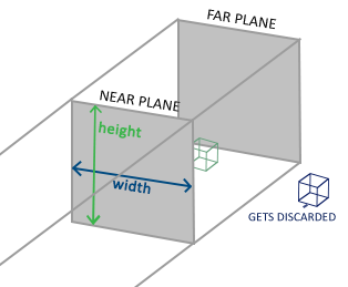
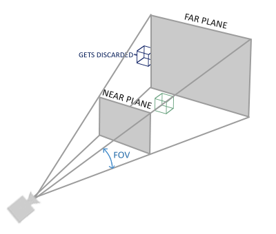
let top = near * Math.tan( _Math.DEG2RAD * 0.5 * this.fov ) / this.zoom;
let height = 2 * top;
let width = this.aspect * height;
let left = - 0.5 * width;
let right = left + width;
let bottom = top - height;

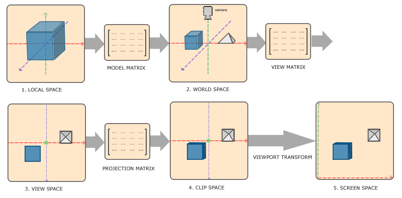
　　对于透视投影，由于计算出的齐次坐标 w 分量显然不为 1.0，所以必须进行透视除法（x,y,z 各分量分别除以 w），得到真正的 3 维坐标。

　　正射投影一般用来模拟 2D 空间，透视投影用来模拟 3D 空间，当透视投影 near 和 far 设置的相差太大时，很容易引发 z-fighting 现象，原因是离近平面越远时，计算出的深度精度越低，three.js 中为解决这一问题，引入了一个 logarithmicDepthBuffer 参数来决定是否开启使用对数函数优化深度计算，具体可看源码中的 logdepthbuf_vertex.glsl.js 和 logdepthbuf_fragment.glsl.js 文件，开启该参数会造成渲染性能下降。

小结

　　\(M_{mvp} = M_{projection}M_{view}M_{model}\)，一个局部坐标 \(V_{local}\) 在经过 MVP 矩阵变换之后可得到裁剪坐标 \(V_{clip} = M_{mvp}V_{local}\) ，在 OpenGL 中，\(V_{clip}\) 会被赋值到顶点着色器中的 gl_Position，并且 OpenGL 会自动进行透视除法和裁剪。

　　3 维中的相机一般可分为两种，第一人称相机（常规 FPS 游戏）和第三人称相机（常规 ARPG 游戏），第一人称相机的特点是灵活，相机往往可以任意改变位置和朝向，所以会对某些人造成一种 “晕 3D” 的现象，而第三人称相机虽然可以改变相机朝向点和位置，但当朝向点和到朝向点的距离一旦固定，则相机只能沿着以朝向点为球心，以到朝向点的距离为半径的球面上运动，这两种相机一般看具体业务需求进行选择。

　　缩放操作是很常规的一种操作，镜头拉近代表放大，拉远代表缩小。在使用透视投影的 3 维场景中，只需要改变相机到朝向点的距离即可简单实现缩放操作，而在使用正射投影的场景中，改变距离并不能实现缩放，而是需要改变 左右上下 四个参数，所以在相机中往往会在引入一个 zoom 的参数，用 左右上下 四个参数分别除以 zoom 得到真正的 左右上下，从而改变 zoom，就可以改变相机参数，进而实现正射投影的缩放。

管线篇

　　渲染管线，图形学中最重要的概念之一，既然称之为管线，自然有像流水线一样的步骤，各个步骤具体做的事情如下：

1. 顶点着色器：负责将顶点数据进行坐标变换，该着色器中一般存在 MVP 矩阵，负责将三维坐标变换为二维坐标，该阶段也可以优化每个点的深度值，以便管线后续进行深度测试，也可以利用光照简单优化每个顶点的颜色；
2. 图元装配：将输入的顶点数据进行组装，形成图元，常见的图元包括：点(GL_POINTS)、线(GL_LINES)、线条(GL_LINE_STRIP)、三角面(GL_TRIANGLES)，在该过程中，一般 GPU 会做一些裁剪和背面剔除等操作，以减少图元的数量，同时完成透视除法以进行屏幕映射；
3. 光栅化：负责计算每个图元到屏幕像素点的映射。光栅化会计算每个图元所覆盖的片元，同时利用顶点属性插值计算每个片元的属性，片元可认为是候选像素，经过后续管线阶段即可变为真正的像素。
4. 片元着色器：将光栅化得到的片元进行颜色计算。图形学中几乎所有的高级特效都会在这一步完成，光照计算，阴影处理，纹理，材质，统统在这一步进行处理；
5. 归属测试：即测试片元所在位置是否位于当前上下文视窗内，若一个显示帧缓冲区视窗被另一个视窗所遮蔽，则剔除该部分片元。
6. 模板测试：即测试片元是否满足一定条件（可大于或小于某个值等），若测试不满足，则剔除该该片元， OpenGL 可自行选择开启或关闭模板测试。
7. 深度测试：用来测试片元的远近，远的片元被遮挡。在深度测试，若两片元深度值接近，则可能会引起 Z-fighting 现象，即像素闪烁，这是因为此时 GPU 无法确定该剔除哪个片元，导致这一帧可能绘制这个片元，下一帧绘制另一个片元。若开启 Alpha 测试，即启用透明度，则会在下一阶段进行 Alpha 混合，从而达到透明效果。
8. 混合：将新生成的片元颜色和帧缓冲区中对应位置的颜色进行混合，得到像素颜色。
9. 抖动：一种以牺牲分辨率为代价来增加颜色表示范围技术，从视觉效果上来看就是颜色过度更平滑。

　　以上这些阶段中，能完全被编程控制的也就顶点着色器和片元着色器两个阶段，其余阶段要么完全无法控制，要么只能通过已有的参数进行设置，当然也可以通过顶点着色器和片元着色器影响余下阶段，顶点着色器和片元着色器也统称 Shader 编程。

　　有时候为了做更好看的特效，需要进行多次渲染，将上一次渲染的结果作为下一次渲染的输入，此时可以将颜色缓冲区作为一张纹理，并构造新的帧缓冲区，将该纹理作为输入，重新放进渲染管线中，这种操作方式也叫后期处理（Post Processing），虽然好看，但对 GPU 的负载很大，需要合理使用。

　　对于渲染管线，Shaun 的理解也就到此为止了，非常粗浅，Shader 也只是刚入门的水平，Shaun 在图形学方面做的更多是降低 Draw-Call 和 CPU 层面的 Tessellation，以及 Geometry 上的事，对纹理材质颜色光照阴影等方面涉及的较少。

后记

　　虽然目前 OpenGL 已停止更新，但学习图形学编程，OpenGL 总是绕不过去（至少暂时以及未来很长一段时间都会是这样），而且图形学基础知识本质都是相同的，不管是 DirectX 还是 Vulkan，变的只是写法形式而已，数学知识总是在那里，两种 shader 也同样需要，所以了解这些东西还是有必要的。

附录

二维图像的图像透视投影变换

　　图像的透视投影变换常用于图像的矫正，OpenCV 中就有现成的 api（getPerspectiveTransform 和 warpPerspective），用于将不规整的四边形区域变换为规整的矩形区域。其基本的数学原理为，先构造一个投影变换等式： \[ \begin{bmatrix} XW \\ YW \\ W \end{bmatrix} = \begin{bmatrix} a & b & c \\ d & e & f \\ g & h & 1 \end{bmatrix} \begin{bmatrix} x \\ y \\ 1 \end{bmatrix} \] 设四边形中四个点分别为 \((X_1, Y_1),(X_2, Y_2),(X_3, Y_3),(X_4, Y_4)\) ，对应矩形中四个点为 \((x_1, y_1),(x_2, y_2),(x_3, y_3),(x_4, y_4)\)。则可构造齐次线性方程组： \[ \begin{bmatrix} x_1 & y_1 & 1 & 0 & 0 & 0 & -X_1x_1 & -X_1y_1 \\ 0 & 0 & 0 & x_1 & y_1 & 1 & -Y_1x_1 & -Y_1y_1 \\ x_2 & y_2 & 1 & 0 & 0 & 0 & -X_2x_2 & -X_2y_2 \\ 0 & 0 & 0 & x_2 & y_2 & 1 & -Y_2x_2 & -Y_2y_2 \\ \vdots & \vdots & \vdots & \vdots & \vdots & \vdots & \vdots & \vdots \\ x_n & y_n & 1 & 0 & 0 & 0 & -X_nx_n & -X_ny_n \\ 0 & 0 & 0 & x_n & y_n & 1 & -Y_nx_n & -Y_ny_n \end{bmatrix} \begin{bmatrix} a \\ b \\ c \\ d \\ e \\ f \\ g \\ h \end{bmatrix} = \begin{bmatrix} X_1 \\ Y_1 \\ X_2 \\ Y_2 \\ \vdots \\ X_n \\ Y_n \end{bmatrix} \] 解这个方程组得到 abcdefg ，使用上面的投影变换等式可计算 \(X = XW / W, Y = YW / W\) ，从而使用插值得到规整矩形图形的各个像素值。

Shader 学习资料

shader 入门书：https://thebookofshaders.com，在线编写 shader ：https://thebookofshaders.com/edit.php

glslsandbox 网站：http://glslsandbox.com/

shadertoy 网站：https://www.shadertoy.com/

threejs shader 系列教程：https://www.cnblogs.com/heymar/category/2432299.html

参考资料

[1] 坐标系统（https://learnopengl-cn.github.io）

[2] WebGL图形系统、渲染管线_郭隆邦技术博客

[3] OpenGL Projection Matrix

[4] WebGL着色器32位浮点数精度损失问题

[5] Transform quadrilateral into a rectangle?

前言

　　最近要改行做大数据相关的东西了，经调研大数据开发的语言还是用 Scala 好，当然 Java 也可以，毕竟都运行在 JVM 上，不过 Java 也有很长时间没用过了，所以对于 Shaun 来说用 Scala 和 Java 的代价是一样的，都需要学习一下，所以决定用对大数据更友好的 Scala。

　　以 Martin Odersky 14 年写的「Scala By Example」为参考，虽然是 14 年的，但 Scala 的基本语法还是没变的，就学习本身而言没问题，毕竟不兼容的只是更上层的 API，Shaun 学习用的 Scala 版本为 2.12.12。Alvin Alexander 的「Scala Cookbook, 2nd Edition」预计今年 8 月会出版，到时可能这本书用来入门更好，但 Shaun 不需要系统的学，就简单的能上手写出比较理想的 Scala 代码就行了。

学习篇

第一章：入门基础

HelloWorld

　　由于「Scala By Example」第一章没啥内容，也为了在正式写 Scala 之前简单熟悉一下，这里先用「A Scala Tutorial for Java Programmers」简单上手一下，首先写个 HelloWorld，具体代码如下：

1
2
3
4
5

object HelloWorld {
    def main(args: Array[String]) {
        println("Hello, world!")
    }
}

　　和 C 语言类似，程序唯一入口函数都是 main 函数，但 Scala 的变量在前，声明的类型在后，相比常规的语言是有点奇怪了，但这种语法规则和 Typescript 一样，所以很容易接受，但其模板的表示就有点奇怪了，Array[String] 表示一个 String 类型的数组，即表示方法为 Array[T]，常规的模板方式为 Array<T> 或 T[]，def 关键字用来定义一个函数，object 用来表示一个单例类，即在定义类的同时，又创建了一个类的实例。Scala 中没有 static 关键字，需要用 static 修饰的都放在 object 中即可。

调用 Java

Scala 中默认已导入 java.lang 中的全部类，但其它类需要显式导入，以格式化输出本地日期为例：

1
2
3
4
5
6
7
8
9
10

import java.util.{Date, Locale}
import java.text.DateFormat._

object LocalDate {
    def main(args: Array[String]) {
        val now = new Date
        val df = getDateInstance(LONG, Locale.CHINA)
        println(df format now) // df format(now)
    }
}

　　Scala 中的导入和 java 中 import 基本一样，但功能更强大，可以使用 {} 导入部分，也使用 _ 导入全部（java 导入全部为 *，这不一样），当一个函数只有一个参数，可以通过 空格+参数 的形式调用，而不需要使用 括号包裹 的形式。这里采用 val 关键字声明的是常量，而要声明变量需要用 var。

对象

Scala 中万物皆对象，一个数字也是一个对象，一个函数也是一个对象，具体如下图：

以简单计时器函数为例：

1
2
3
4
5
6
7
8
9
10
11
12
13
14
15
16
17
18
19

object Timer {
    def oncePerSecond(callback: () => Unit) {
        while (true) {
            callback();
            Thread sleep 1000;
        }
    }

    def timeFiles() {
        println("time files like an arrow...");
    }

    def main(args: Array[String]) {
        // oncePerSecond(timeFiles);
        oncePerSecond(() => {
            println("time files like an arrow...");
        });
    }
}

　　这个和 Typescript 函数式编程的用法基本差不多，唯一不同这里声明的函数返回的是 Unit ，这个 Unit 可认为是无返回的函数，大部分情况等同于 void，在 Scala 中真正的没有值指的是 Nothing。

类

Scala 中同样有类，具体代码示例如下：

1
2
3
4
5
6
7
8
9
10
11
12
13
14
15
16

class Complex(real: Double, imaginary: Double) {
    // def re() = real;
    // def im() = imaginary;
    def re = real;
    def im = imaginary;
    
    override def toString(): String = "" + re + (if (im < 0) "" else "+") + im + "i";
}

object ComplexNumbers {
    def main(args: Array[String]) {
        val c = new Complex(1.2, -3.4);
        // println("real part: " + c.re() + " imaginary part: " + c.im());
        println(c.toString());
    }
}

　　在 Scala 中所有类都会继承某个父类，若没有显式声明父类，则默认继承 scala.AnyRef 类，如上面的 Complex 类，若需要覆盖父类的函数，则需要在函数声明前加上 override 关键字。当函数没有参数时，可以不用加括号，在调用时也不用加括号，如上面示例的注释和非注释的代码。

模式匹配与条件类

　　接下来用 Scala 来写一个树结构表示表达式的示例代码，树的非叶节点表示操作符，叶子节点表示数值（这里为常量或变量），具体代码如下：

1
2
3
4
5
6
7
8
9
10
11
12
13
14
15
16
17
18
19
20
21
22
23
24
25
26
27
28
29

abstract class Tree
case class Sum(l: Tree, r: Tree) extends Tree
case class Var(n: String) extends Tree
case class Const(v: Int) extends Tree

object Expression {
    type Environment = String => Int

    def eval(t: Tree, env: Environment): Int = t match {
        case Sum(l, r) => eval(l, env) + eval(r, env)
        case Var(n) => env(n)
        case Const(v) => v
    }

    def derive(t: Tree, v: String): Tree = t match {
        case Sum(l, r) => Sum(derive(l, v), derive(r, v))
        case Var(n) if (v == n) => Const(1)
        case _ => Const(0)
    }

    def main(args: Array[String]) {
        val exp: Tree = Sum(Sum(Var("x"), Var("x")), Sum(Const(7), Var("y"))) 
        val env: Environment = {case "x" => 5 case "y" => 7}
        println("Expression: " + exp)
        println("Evalution with x=5, y=7: " + eval(exp, env))
        println("Derivative relative to x:\n" + derive(exp, "x"))
        println("Derivative relative to y:\n" + derive(exp, "y"))
    }
}

　　该示例主要用来说明两种 case 关键字，分别为：case class 和 ... match case ...，前者可认为是一个结构体，实例化时可以省略 new 关键字，参数有默认的 getter 函数，整个 case class 有默认的 equals 和 hashCode 方法实现，通过这两个方式可实现根据值判断类的两个实例是否相等，而不是通过引用，条件类同样有默认的 toString 方法实现；后者可认为是一种特殊的 switch case ，只不过 case 的判定和执行是函数式的，case class 可直接参与 match case 的判定（判定是不是属于该类）。第 7 行中有个 type 关键字，可认为是定义了一种新的类型（不是数据类型），示例中是函数类型，通过这个 type ，可直接将字符串映射为整型，23 行中将这个 type 与 case 结合使用，定义多个字符串映射多个整型的变量。第 18 行中有个 _ ，这是 scala 中的通配符，不同的语义下表示的含义不同，这里的含义是指，当上面的模式都不匹配时，将执行这个，相当于 switch case 中的 default。

Scala 中的 trait

　　简单理解就是 Java 中的 Interface（接口），Scala 中没有 interface 关键字，但是 trait 比 Interface 的功能更多，其中可直接定义属性和方法的实现，Scala 中可通过 trait 来实现多重继承。下面的示例用 trait 简单实现了一个比较接口：

1
2
3
4
5
6
7
8
9
10
11
12
13
14
15
16
17
18
19
20
21
22
23
24
25
26
27
28
29
30
31
32
33
34
35
36
37
38
39
40

trait Ord {
    def <(that: Any): Boolean
    def <=(that: Any): Boolean = (this < that) || (this == that)
    def >(that: Any): Boolean = !(this <= that)
    def >=(that: Any): Boolean = !(this < that)
}

class Date(y: Int, m: Int, d: Int) extends Ord {
    def year = y
    def month = m
    def day = d

    override def toString(): String = year + "-" + month + "-" + day

    override def equals(that: Any): Boolean = {
        that.isInstanceOf[Date] && {
            val o = that.asInstanceOf[Date]
            o.day == day && o.month == month && o.year == year
        }
    }

    def <(that: Any): Boolean = {
        if (!that.isInstanceOf[Date]) {
            sys.error("cannot compare " + that + " and a Date")
        }

        val o = that.asInstanceOf[Date]
        (year < o.year) || (year == o.year && (month < o.month || (month == o.month && day < o.day)))
    }
}

object Comparable {
    def main(args: Array[String]) {
        val d1 = new Date(2021, 1, 3);
        val d2 = new Date(2021, 1, 3);

        println(d1 < d2)
        println(d1 <= d2)
    }
}

　　比较关系一般只需要确定 小于 和 等于 关系即可，其它关系都可由这两关系推出来，由于等于方法默认存在于所有对象中，所以只需要重写小于即可， 其它的比较方法都可以在 trait 中定义好。在上面的示例中有两个函数 isInstanceOf 和 asInstanceOf，前者用来判断对象是否是指定类型，后者用来将对象转换为指定类型，一般用在将父类转为子类时，在使用 asInstanceOf 之前一般需要先使用 isInstanceOf。

泛型

　　这东西没啥好说的，基本有编程经验的或见过或用过，只是 Scala 的泛型语法确实有点奇怪就是了，可能也是为了函数式那些乱七八糟的操作符，具体示例代码如下：

1
2
3
4
5
6
7
8
9
10
11
12
13
14
15

class Reference[T] {
    private var contents: T = _
    def set(value: T) {
        contents = value
    }
    def get: T = contents
}

object IntegerReference {
    def main(args: Array[String]) {
        val cell = new Reference[Int]
        cell.set(13)
        println("Reference contains the half of " + (cell.get * 2))
    }
}

　　这里同样有个 _，这里表示的是默认值，对于数字类型来说是 0，对于 boolean 来说是 false，对于 Unit（函数签名）来说是()（无参数无返回），对于其他来说是 null。

简单的了解 Scala 就到这里了。

第二章：快排

开场就是一个快排，示例代码如下：

1
2
3
4
5
6
7
8
9
10
11
12
13
14
15
16
17
18
19
20
21
22
23
24
25
26
27
28
29
30
31
32
33
34
35
36
37
38
39
40
41
42
43
44

object QuickSort {
    def qSort(xs: Array[Int]) {
        def swap(i: Int, j: Int) {
            val t = xs(i); xs(i) = xs(j); xs(j) = t;
        }

        def sort(l: Int, r: Int) {
            val pivot = xs(l);
            var i = l+1; var j = r;
            while (i < j) {
                while (i <= r && xs(i) < pivot) i += 1;
                while (j > l && xs(j) > pivot) j -= 1;

                if (i < j) {
                    swap(i, j);
                    i += 1;
                    j -= 1;
                }

                if (i > j) {
                    i = j;
                }
            }
            while (i > l && xs(i) > pivot) {
                i -= 1; j -= 1;
            }
            swap(i, l);

            if (l < j-1) sort(l, j-1);
            if (j+1 < r) sort(j+1, r);
        }

        sort(0, xs.length-1);
    }

    def main(args: Array[String]) {
        // val xs = Array(4, 1, 2, 5, 6);
        // val xs = Array(1, 2, 4, 4, 55, 5, 6);
        // val xs = Array(55, 6, 6);
        val xs = Array(4, 1, 5, 7,7,7,7, 2, 6);
        qSort(xs);
        println(xs.mkString(" "))
    }
}

　　从这段快排代码可看出，Scala 支持函数嵌套和闭包，即在函数内部定义子函数，子函数可直接使用父函数的变量，同时，这里也简单说明一下 Scala 中数组的一些使用方法，用下标取数组元素时使用的是小括号 ()，而不是其它语言常见的中括号 []。当然 Scala 作为一种函数式语言，提供了非常多的函数式操作符，这篇也只会简单介绍。

第三章：Actor

　　Actor，Scala 中的多线程编程模型，下方的示例代码在 Scala 2.11 及之后的版本无法运行，因为 Actor 已从 Scala 库独立出来，见 object-actors-is-not-a-member-of-package-scala。

1
2
3
4
5
6
7
8
9
10
11
12
13
14
15
16
17
18
19
20
21
22
23
24
25
26
27
28
29
30
31
32
33
34
35
36
37
38
39
40
41
42
43
44
45
46
47
48
49
50
51
52
53
54
55
56
57
58
59
60
61
62
63
64
65
66
67
68
69
70
71
72
73
74
75
76
77
78

import scala.actors.Actor

abstract class AuctionMessage
case class Offer(bin: Int, client: Actor) extends AuctionMessage
case class Inquire(client: Actor) extends AuctionMessage

abstract class AuctionReply
case class Status(asked: Int, expire: Date) extends AuctionReply
case object BestOffer extends AuctionReply
case class BeatenOffer(maxBid: Int) extends AuctionReply
case class AuctionConCluded(seller: Actor, client: Actor) extends AuctionReply

case object AuctionFailed extends AuctionReply
case object AuctionOver extends AuctionReply


class Auction(seller: Actor, minBid: Int, closing: Date) extends Actor {
    val timeToShutdown = 36000000 // msec
    val bidIncrement = 10

    def act() {
        var maxBid = minBid - bidIncrement
        var maxBidder: Actor = null
        var running = true

        while (running) {
            receiveWithin ((closing.getTime() - new Date().getTime())) {
                case Offer(bid, client) => {
                    if (bid >= maxBid + bidIncrement) {
                        if (maxBid >= minBid)   maxBidder ! BeatenOffer(bid)
                        maxBid = bid; maxBidder = client; client ! BestOffer
                    } else {
                        client ! BeatenOffer(maxBid)
                    }
                }
                case Inquire(client) => {
                    client ! BeatenOffer(maxBid)
                }
                case TIMEOUT => {
                    if (maxBid >= minBid) {
                        val reply = AuctionConCluded(seller, maxBidder)
                        maxBidder ! reply; seller ! reply
                    } else {
                        seller ! AuctionFailed
                    }

                    receiveWithin(timeToShutdown) {
                        case Offer(_, client) => client ! AuctionOver
                        case TIMEOUT => running = false
                    }
                }
            }
        }
    }
}

class HelloActor extends Actor {
    def act() {
        while (true) {
            receive {
                case name: String => println("Hello, " + name)
            }
        }
    }
}

object AuctionService {
    def main(args: Array[String]) {
        val seller: Actor = new HelloActor
        val client: Actor = new HelloActor
        val minBid = 10
        val closing = new Date()

        val helloActor = new HelloActor
        helloActor.start()
        helloActor ! "leo"
    }
}

　　通过重写 Actor 中的 act 方法即可简单的实现多线程编程，Actor 中有个特殊的标识符 !，该符号其实是是一种缩写，即可将 helloActor.!("leo") 缩写为 helloActor ! "leo"，代表将数据传递给 Actor，由 Actor 内部的 receive case 接受数据并处理，当然也可通过 receiveWithin 控制数据传递时间，若超时，则默认触发 TIMEOUT 处理模式。

第四章：表达式与简单函数

该章主要有两个例子：1、牛顿法求平方根；2、尾递归，具体如下：

1
2
3
4
5
6
7
8
9
10
11
12
13
14
15
16
17
18
19
20
21
22
23
24
25
26
27
28
29
30
31
32
33
34
35
36
37
38
39
40
41
42
43
44
45
46
47

object Sqrt {
    def sqrt(x: Double): Double = {
        def sqrtIter(guess: Double, x: Double): Double = {
            if (isGoodEnough(guess, x)) guess
            else sqrtIter(improve(guess, x), x)
        }

        def improve(guess: Double, x: Double) = {
            (guess + x / guess) / 2
        }

        def isGoodEnough(guess: Double, x: Double) = (guess * guess - x).abs < 0.001    // guess * guess == x

        sqrtIter(1.0, x)
    }
}

object TailRecursion {
    def gcd(a: Int, b: Int): Int = if (b == 0) a else gcd(b, a % b)

    def facorial(n: Int): Int = if (n == 0) 1 else n * facorial(n-1)

    def facorialTail(n: Int): Int = {
        def facorialIter(n: Int, res: Int): Int = {
            if (n == 0) res
            else facorialIter(n-1, res * n)
        }

        facorialIter(n, 1)
    }
}

object SimpleFunc {
    def main(args: Array[String]) {
        val sqrtValue = Sqrt.sqrt(0.01)
        println(sqrtValue)

        val gcdValue = TailRecursion.gcd(14,21)
        println(gcdValue)

        val facorialValue = TailRecursion.facorial(5)
        println(facorialValue)

        val facorialTailValue = TailRecursion.facorialTail(5)
        println(facorialTailValue)
    }
}

　　由于并没有引入新的语法，就简单聊聊这两个例子吧。牛顿法求平方根主要在于构造一个特殊的二分函数 \(y_{i+1} = (y_i + x / y_i)/2, i=0,1,2,3,..., y_0=1\) ，如此迭代，直到 \(|y_i^2-x| < \epsilon\) ，得到 \(y_i\) 即为 x 的平方根，更朴素一点的求多次方根就是利用二分法，分 [0, 1] 和 [1, +∞] 两个区间即可，对应从 [x, 1] 和 [1, x] 开始二分取值。至于尾递归，以前简单的写过一点，即最后递归调用原函数时，原函数不会再参与任何计算表达式。尾递归的好处在于当编译器或解释器支持尾递归时，将不会产生普通递归时的压栈操作，即不用担心递归层次太深，尾递归将类似循环迭代处理。

第五章：高阶函数

　　高阶函数（First-Class Functions），支持以函数作为参数或返回值，也可将函数赋值给其它变量，由此也可引出闭包和柯里化，闭包是指将内嵌函数作为返回值，而柯里化是指将多个参数分解为独立参数传递给函数，如：\(f(args_1,args_2,...,args_n)=f(args_1)(args_2)(...)(args_n)\)。下面以求函数的不动点为例：

1
2
3
4
5
6
7
8
9
10
11
12
13
14
15
16
17
18
19

object FirstClassFunctions {
    val tolerance = 0.0001
    def isCloseEnough(x: Double, y: Double) = ((x-y) / x).abs < tolerance
    def fixedPoint(f: Double => Double)(firstGuess: Double) = {
        def iterate(guess: Double): Double = {
            val next = f(guess)
            if (isCloseEnough(guess, next)) next
            else iterate(next)
        }
        iterate(firstGuess)
    }

    def averageDamp(f: Double => Double)(x: Double) = (x + f(x)) / 2
    def sqrt(x: Double) = fixedPoint(averageDamp(y => x/y))(1.0)

    def main(args: Array[String]) {
        println(sqrt(0.01));
    }
}

　　该示例简单明了的展示了 Scala 中匿名函数，函数柯里化以及闭包。

第六章：类和对象

直接看下面的有理数示例吧，

1
2
3
4
5
6
7
8
9
10
11
12
13
14
15
16
17
18
19
20
21
22
23
24
25
26
27
28
29
30
31
32
33
34
35

// 主构造函数
class Rational(n: Int, d: Int) extends AnyRef {
    private def gcd(x: Int, y: Int): Int = {
        if (x == 0) y
        else if (x < 0) gcd(-x, y)
        else if (y < 0) -gcd(x, -y)
        else gcd(y % x, x)
    }
    private val g = gcd(n, d)

    // 构造函数重载（辅助构造函数）
    def this() {
        this(0, 0)  // 调用主构造函数
    }

    val number: Int = if (g != 0) n / g else 0
    val denom: Int = if (g != 0) d / g else 0

    def +(that: Rational) = new Rational(number * that.denom + that.number * denom, denom * that.denom)
    def -(that: Rational) = new Rational(number * that.denom - that.number * denom, denom * that.denom)
    def *(that: Rational) = new Rational(number * that.number, denom * that.denom)
    def /(that: Rational) = new Rational(number * that.denom, denom * that.number)

    def toNumber: Double = if (denom != 0) number.toDouble / denom else 0.0

    override def toString = "" + number + "/" + denom
}

object Rational {
    def main(args: Array[String]) {
        val rational = new Rational(2,1) / new Rational()
        println(rational.toNumber);
        println(rational.toString);
    }
}

　　从有理数这个示例可以看出，Scala 的类支持操作符重载，也支持构造函数重载，同样支持继承，多继承也是支持的，每个父类用 with 关键字分隔就行。

第七章：条件类和模式匹配

大致和第一章内容差不多，就不重复写了。

第八章：泛型

　　大致也和第一章内容差不多，值得一提的书中实现的泛型栈本质是一个链表，实现方法挺有意思的。通过 <: 标识符可约束泛型的类型，如 [T <: P[T]] 表明泛型 T 必须类型 P 的子类型。而标识符 <% 比 <: 约束性弱一点，只要 T 能够通过隐式类型变换为 P 即可。若想约束为父类型，则需使用 >: 标识符。

　　Scala 中有一种特殊的泛型，就是变化型注解，trait List[+T] 代表协变，表示当 B 类型是 A 类型子类时，List[B] 也可认为是 List[A] 的子类；trait List[-T] 代表逆变，当 B 类型是 A 类型子类时，List[B] 可认为是 List[A] 的父类。

　　Scala 中同样有元组，使用时也很方便，简单使用直接用括号声明即可，如 def divmod(x: Int, y: Int): (Int, Int) = (x / y, x % y)，该函数即返回一个元组，也可声明一个元组 case class Tuple2[A, B](_1: A, _2: B)，若需要取元组的元素可通过 _i 的方式，如 val xy = divmod(3, 4); xy._1; xy._2;，也可通过 match-case 语句取，如 xy match { case (n, d) => println("quotient: " + n + ", rest: " + d) }。

第九章：List

　　Scala 中的 List 其实是数组结构，并且是不可变的，可认为是 C++ 里的静态数组，不能往其中添加或删除元素，下面用数组排序示例下 List 的用法：

1
2
3
4
5
6
7
8
9
10
11
12
13
14
15
16
17
18
19
20
21
22
23
24
25
26
27
28
29
30
31
32
33
34
35
36

object Sort {
    def insertSort(xsl: List[Int]): List[Int] = {
        def insert(x: Int, xs: List[Int]): List[Int] = {
            xs match {
                // case Nil => List(x)
                case List() => List(x)
                case y :: ys => if (x <= y) x :: xs else y :: insert(x, ys)
            }
        }

        if (xsl.isEmpty) Nil
        else insert(xsl.head, insertSort(xsl.tail))
    }

    def mergeSort[A](less: (A, A) => Boolean)(xs: List[A]): List[A] = {
        def merge(xs1: List[A], xs2: List[A]): List[A] = {
            if (xs1.isEmpty) xs2
            else if (xs2.isEmpty) xs1
            else if (less(xs1.head, xs2.head)) xs1.head :: merge(xs1.tail, xs2)
            else  xs2.head :: merge(xs1, xs2.tail)
        }

        val n = xs.length / 2
        if (n == 0) xs
        else merge(mergeSort(less)(xs take n), mergeSort(less)(xs drop n))
    }

    def main(args: Array[String]) {
        val xs = List(4, 1, 5, 7,7,7,7, 2, 6);
        // val xs = 3::2::1::1::Nil;
        println(xs(0), xs(1), xs(xs.length-1)) // (4,1,6)
        // val ys = insertSort(xs);
        val ys = mergeSort((x: Int, y: Int) => x > y)(xs);
        println(ys.mkString(" "))
    }
}

　　List 中有两个操作符非常类似，即 :: 和 :::， 前者用于 List 中的元素和 List 连接，即创建一个新 List，新 List 为原 List 头插入元素后的 List，后者用于连接两个 List，即创建一个新 List ，新 List 为将第二个 List 的元素全部放入第一个 List 尾部的 List。字符 Nil 代表空 List 和 List() 等效，head 方法返回 List 的第一个元素，tail 方法返回除第一个元素之外的其它所有元素，还是一个 List，isEmpty 方法当 List 为空时返回 true。List 的 case-match 方法中，case y :: ys 其中 y 代表 xs.head，ys 代表 xs.tail。(xs take n) 表示取 List 前 n 个元素，(xs drop n) 表示取 List 前 n 个元素之外的元素，即与 (xs take n) 取得元素正好互补，而 (xs split n) 返回一个元组，元组中第一个元素为 (xs take n)，第二个元素为 (xs drop n)。关于 List 还有些更高阶得方法：filter，map, flatMap, reduceRight, foldRight 等方法就不继续写了。至于动态 List 可用 ListBuffer 结构，当然 Scala 中直接用 Seq 作为返回值和参数一般会更好些。

第十章：序列理解

　　Scala 中用来做序列理解的表达式是 For-Comprehensions，具体示例如下：for (p <persons if p.age > 20) yield p.name 相当于 persons filter (p => p.age > 20) map (p => p.name)，可以简单认为 for-yield 方法是 filter 和 map 的集合体。下面具体用个 N-皇后（特例是 8 皇后）的示例来具体说明：

1
2
3
4
5
6
7
8
9
10
11
12
13
14
15
16
17
18
19
20
21
22
23
24
25
26
27
28
29
30
31
32

object NQueen {
    def queens(n: Int): List[List[Int]] = {
        def isSafe(col: Int, queenList: List[Int], delta: Int): Boolean = {
            val curRow = queenList.length-1 + delta
            for (row <- List.range(0, queenList.length)) {
                val queenCol = queenList(row)
                val queenRow = queenList.length-1 - row

                if (queenCol == col) return false
                if (queenRow == curRow) return false
                if ((queenCol - col).abs == (queenRow - curRow).abs) return false
            }
            true
        }

        def placeQueens(k: Int): List[List[Int]] = {
            if (k == 0) List(List())
            else for { 
                queens <- placeQueens(k-1);
                column <- List.range(0, n);
                if isSafe(column, queens, 1) 
            } yield column :: queens
        }
        
        placeQueens(n)
    }

    def main(args: Array[String]) {
        val queenList = queens(8);
        println("queenCount: " + queenList.length)  // 92
    }
}

for-yield 表达式中 for 中可以写多条语句，代表多重循环，第 5 行的 for 代表 for 循环，<- 表示取 List 中的元素。

　　剩下的几章就没啥特别要写的，重点就两个特性，一个是 Stream ，一个 Lazy，Stream 和 List 有点类似，主要区别在于 Stream 是即时返回的，算一个返回一个，而 List 一般是全部计算完再返回一个 List；Lazy 一般用作常量的修饰符，主要作用是只用该常量被用到时才赋值，否则一直为空，有点类似常见的先判空再取值的封装。

后记

　　曾看到过通过刷题去学习新语言的方式，一直都以为很粗暴，但这次照着「Scala By Example」敲下来，感觉还挺有效的，同时也巩固了一下基本的算法知识，后续再把 twitter 的 「Effective Scala」再看一下应该就差不多了。

前言

　　记录一下服务器问题排查常用的一些命令。

常用篇

Linux

1
2
3
4
5
6
7
8
9
10
11
12
13
14
15
16
17
18
19
20
21
22
23
24
25
26
27
28
29
30
31
32
33
34
35
36
37
38
39
40
41
42
43
44
45
46
47
48
49
50
51
52
53
54
55
56
57
58
59
60
61
62
63
64
65
66
67

# 只列出含 XXX 的文件
ll | grep "XXX"

# 按列显示文件名
ls -1
ls -l | grep ^[^d] | awk '{print $9}'

# 返回进入当前目录之前的目录
cd -

# 在文件中查找带 XXX 的行，并输出到 /tmp/99
fgrep "XXX" a.txt > /tmp/99

# 在当前文件夹中查找带 XXX 的行，并输出到 /tmp/99
fgrep "XXX" -r ./* > /tmp/99

# 显示前5行
head -n 5 a.txt

# 显示倒数第5行
tail -n 5 a.txt

# 显示第5行至末尾
tail -n +5 a.txt

#  提取第二行 [linux系统中sed命令输出指定的行](https://www.cnblogs.com/superbaby11/p/16556602.html)
sed -n '2p' a.txt

# 以;分隔每一行，并提取第一列和第三列
awk -F ';' '{print $1,$3}' a.txt

# 以:分隔每一行，并提取第一列和第三列
awk -F '[:]' '{print $1,$3}' a.txt

# 查看 8080 端口占用
lsof -i:8080
netstat -tnlp | grep :8080

# 查看系统运行状态
top

# 查看一定时间内进程cpu占用情况
pidstat

# 查看运行进程
ps -ef

# 查看postgres数据库连接状态，并按cpu使用率排序
ps -aux | grep postgres | sort -nrk 3,3

# 查看磁盘占用大小
du -sh *

# 查看磁盘剩余空间
df -h

# 查看程序被 killed 的原因
dmesg -T | egrep -i -B100 'killed process'
# dmesg 的时间可能不对，可以结合 /var/log/messages 一起看，[dmesg 时间误差现象](https://www.cnblogs.com/edisonfish/p/17283958.html)
cat /var/log/messages | grep "Killed process"

# 查看 url 请求时间
curl -o /dev/null -s -w %{time_namelookup}:%{time_connect}:%{time_starttransfer}:%{time_total} [url]

# 查看硬盘序列号
sudo lshw -class disk | grep serial

正则表达式

常用正则：i Hate Regex

1
2
3
4
5
6
7
8
9
10
11

// 匹配 hello 之前的字符
(.+(?=hello))

// 匹配其他数字和英文字母但不匹配结尾的 2
([a-zA-Z_0-9]+[^2])

// 提取包含test以及time后的数字
test[a-zA-Z0-9\-\_\=\|\ ]*time=([\d+])

// 提取中括号里的内容
[\[](.*?)[\]]

工具

• crontab：设置定时任务工具；
• Socat：网络工具（透明代理，端口转发，文件传输等），新版瑞士军刀：socat

服务器之间文件传输

参考资料：Linux下的SCP指令详解

1
2
3
4
5
6
7
8
9
10
11
12
13
14
15
16
17

# 本地主机传输文件到远程主机
scp [本地文件路径] [用户名]@[远程主机IP地址]:[目标路径]
# eg:
scp file.txt user@example.com:/home/user/

# 远程主机传输文件到本地主机
scp [用户名]@[远程主机IP地址]:[远程文件路径] [本地目标路径]
# eg:
scp user@example.com:/home/user/file.txt /path/to/local/

# 传输本地主机整个目录到远程主机
scp -r [本地目录路径] [用户名]@[远程主机IP地址]:[目标路径]
# eg:
scp -r directory/ user@example.com:/home/user/

# 若远程主机的SSH服务器端口不是默认的22端口，则需要指定端口号
scp -P [端口号] [本地文件路径] [用户名]@[远程主机IP地址]:[目标路径]

PostgreSQL

编译安装

参考自：【CentOS7】PostgreSQL-10.3的安装

1. 安装编译工具：

   1	yum install -y vim lrzsz tree wget gcc gcc-c++ readline-devel zlib-devel

2. 进入/usr/local/目录下：cd /usr/local

3. 下载 tar 包：curl -O https://ftp.postgresql.org/pub/source/v16.2/postgresql-16.2.tar.gz

4. 解压：tar -xzvf postgresql-16.2.tar.gz

5. 编译安装：

   1 2 3 4 5

   cd /usr/local/postgresql-16.2 ./configure --prefix=/usr/local/pgsql-16.2 # /usr/local/pgsql-16.2 为安装目录 make && make install # Two thousand years later，出现「PostgreSQL installation complete.」代表安装成功

6. 配置系统环境变量：vi /etc/profile

   1 2 3 4 5 6

   ... # /etc/profile 文件末尾添加 export PGHOME=/usr/local/pgsql-16.2 export PGDATA=$PGHOME/data export LD_LIBRARY_PATH=$PGHOME/lib:$LD_LIBRARY_PATH export PATH=$PGHOME/bin:$PATH

7. 使配置文件立即生效：source /etc/profile

8. 创建数据库用户：useradd -m -d /home/postgres postgres

9. 切换到数据库用户：su postgres

10. 初始化数据库：pg_ctl init -D /home/postgres/db_data

11. 启动数据库：pg_ctl start -D /home/postgres/db_data

自启动设置

复制 PostgreSQL 自启动文件：cp /usr/local/postgresql-16.2/contrib/start-scripts/linux /etc/init.d/postgresql

修改自启动文件：vi /etc/init.d/postgresql，

1
2
3
4
5
6
7
8
9
10
11
12
13
14
15
16
17
18
19
20
21
22
23
24
25
26
27
28
29
30
31
32
33
34
35
36
37
38
39
40
41
42
43
44
45
46
47
48
49
50
51
52
53
54
55
56
57
58
59
60
61
62
63
64
65
66
67
68
69
70
71
72
73
74
75
76
77
78
79
80
81
82
83
84
85
86
87
88
89
90
91
92
93
94
95
96
97
98
99
100
101
102
103
104
105
106
107
108
109
110
111
112
113
114
115
116
117
118
119
120
121
122
123
124
125
126

#! /bin/sh

# chkconfig: 2345 98 02
# description: PostgreSQL RDBMS

# This is an example of a start/stop script for SysV-style init, such
# as is used on Linux systems.  You should edit some of the variables
# and maybe the 'echo' commands.
#
# Place this file at /etc/init.d/postgresql (or
# /etc/rc.d/init.d/postgresql) and make symlinks to
#   /etc/rc.d/rc0.d/K02postgresql
#   /etc/rc.d/rc1.d/K02postgresql
#   /etc/rc.d/rc2.d/K02postgresql
#   /etc/rc.d/rc3.d/S98postgresql
#   /etc/rc.d/rc4.d/S98postgresql
#   /etc/rc.d/rc5.d/S98postgresql
# Or, if you have chkconfig, simply:
# chkconfig --add postgresql
#
# Proper init scripts on Linux systems normally require setting lock
# and pid files under /var/run as well as reacting to network
# settings, so you should treat this with care.

# Original author:  Ryan Kirkpatrick <pgsql@rkirkpat.net>

# contrib/start-scripts/linux

## EDIT FROM HERE

###### 上面不改 #####################
# Installation prefix
prefix=/usr/local/pgsql-16.2

# Data directory
PGDATA="/home/postgres/db_data"
###### 下面不改 #####################

# Who to run postgres as, usually "postgres".  (NOT "root")
PGUSER=postgres

# Where to keep a log file
PGLOG="$PGDATA/serverlog"

# It's often a good idea to protect the postmaster from being killed by the
# OOM killer (which will tend to preferentially kill the postmaster because
# of the way it accounts for shared memory).  To do that, uncomment these
# three lines:
#PG_OOM_ADJUST_FILE=/proc/self/oom_score_adj
#PG_MASTER_OOM_SCORE_ADJ=-1000
#PG_CHILD_OOM_SCORE_ADJ=0
# Older Linux kernels may not have /proc/self/oom_score_adj, but instead
# /proc/self/oom_adj, which works similarly except for having a different
# range of scores.  For such a system, uncomment these three lines instead:
#PG_OOM_ADJUST_FILE=/proc/self/oom_adj
#PG_MASTER_OOM_SCORE_ADJ=-17
#PG_CHILD_OOM_SCORE_ADJ=0

## STOP EDITING HERE

# The path that is to be used for the script
PATH=/usr/local/sbin:/usr/local/bin:/sbin:/bin:/usr/sbin:/usr/bin

# What to use to start up postgres.  (If you want the script to wait
# until the server has started, you could use "pg_ctl start" here.)
DAEMON="$prefix/bin/postgres"

# What to use to shut down postgres
PGCTL="$prefix/bin/pg_ctl"

set -e

# Only start if we can find postgres.
test -x $DAEMON ||
{
	echo "$DAEMON not found"
	if [ "$1" = "stop" ]
	then exit 0
	else exit 5
	fi
}

# If we want to tell child processes to adjust their OOM scores, set up the
# necessary environment variables.  Can't just export them through the "su".
if [ -e "$PG_OOM_ADJUST_FILE" -a -n "$PG_CHILD_OOM_SCORE_ADJ" ]
then
	DAEMON_ENV="PG_OOM_ADJUST_FILE=$PG_OOM_ADJUST_FILE PG_OOM_ADJUST_VALUE=$PG_CHILD_OOM_SCORE_ADJ"
fi


# Parse command line parameters.
case $1 in
  start)
	echo -n "Starting PostgreSQL: "
	test -e "$PG_OOM_ADJUST_FILE" && echo "$PG_MASTER_OOM_SCORE_ADJ" > "$PG_OOM_ADJUST_FILE"
	su - $PGUSER -c "$DAEMON_ENV $DAEMON -D '$PGDATA' >>$PGLOG 2>&1 &"
	echo "ok"
	;;
  stop)
	echo -n "Stopping PostgreSQL: "
	su - $PGUSER -c "$PGCTL stop -D '$PGDATA' -s"
	echo "ok"
	;;
  restart)
	echo -n "Restarting PostgreSQL: "
	su - $PGUSER -c "$PGCTL stop -D '$PGDATA' -s"
	test -e "$PG_OOM_ADJUST_FILE" && echo "$PG_MASTER_OOM_SCORE_ADJ" > "$PG_OOM_ADJUST_FILE"
	su - $PGUSER -c "$DAEMON_ENV $DAEMON -D '$PGDATA' >>$PGLOG 2>&1 &"
	echo "ok"
	;;
  reload)
	echo -n "Reload PostgreSQL: "
	su - $PGUSER -c "$PGCTL reload -D '$PGDATA' -s"
	echo "ok"
	;;
  status)
	su - $PGUSER -c "$PGCTL status -D '$PGDATA'"
	;;
  *)
	# Print help
	echo "Usage: $0 {start|stop|restart|reload|status}" 1>&2
	exit 1
	;;
esac

exit 0

接下来有两种方式：

一种是直接执行：cd /etc/rc.d/init.d/ && chkconfig --add postgresql；

一种是修改 /etc/rc.d/rc.local 文件：vi /etc/rc.d/rc.local，

1
2
3
4
5
6
7
8
9
10
11
12
13
14
15
16
17
18
19
20
21
22
23
24

#!/bin/bash
# THIS FILE IS ADDED FOR COMPATIBILITY PURPOSES
#
# It is highly advisable to create own systemd services or udev rules
# to run scripts during boot instead of using this file.
#
# In contrast to previous versions due to parallel execution during boot
# this script will NOT be run after all other services.
#
# Please note that you must run 'chmod +x /etc/rc.d/rc.local' to ensure
# that this script will be executed during boot.
 
exec 2> /tmp/rc.local.log      # send stderr from rc.local to a log file
exec 1>&2                      # send stdout to the same log file
echo "rc.local starting..."        # show start of execution
set -x

touch /var/lock/subsys/local

cd /etc/rc.d/init.d/
sudo sh postgresql start &      # 以root执行，不然可能会出现权限错误，&表示后台执行
 
# 脚本执行完后也给个日志
echo "rc.local completed"

添加可执行权限：chmod a+x /etc/rc.d/rc.local，最后查看一下 rc.local 服务是否启动：

1
2
3
4
5
6
7
8

systemctl status rc-local.serives
 
# 启动命令
systemctl enable rc-local.service
systemctl start rc-local.service
 
# 查看数据库服务
ps -ef | grep postgres

若要在容器中设置自启动，在没给容器提权的情况下，则需要第三种方式：将 /etc/rc.d/init.d/postgresql 放进 /root/.bashrc 中启动，vi /root/.bashrc，

1
2
3
4
5